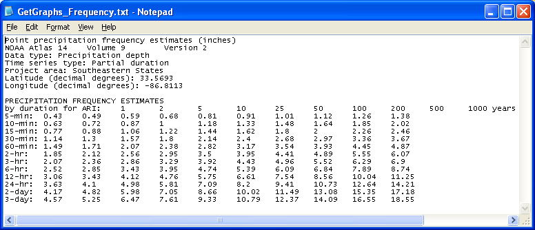
Update 3/4/2013--GetGraphs can now lookup the rainfall
frequencies for unit-values, hourlys, and daily's for display. The needed
rainfall frequency table 'GetGraphs_Frequency.txt' example is
in the current GetRealtime_setup.exe download. The format is easy if you use
NOAA Atlas 14:
http://hdsc.nws.noaa.gov/hdsc/pfds/pfds_map_cont.html?bkmrk=al
Use the submit button for 'Estimates from the table in csv format:' and open in
Excel and save as tab delimited text file as shown here:
The GetGraphs_Setup.txt needs to be edited to look like this with the ending
'-1' for just the unit or hourly values and daily or ending '-2' for a
full frequency curve of the actual maximum depths for the durations :
5 ;Frequencies; 10 ; 10 ;-1
1 ; 10612 ;Rainfall Frequency;Hueytown, AL; 0;1;0; 6335701 ; 9684176 ;
16711680 ; 255 ;;;; 0 ;-2
2 ; 10613 ;Rainfall Frequency;Bham Airport; 0;1; 0; 6335701 ;
9684176 ; 16711680 ; 255 ;;;; 0 ;-1
3 ;
4 ;
5 ;
6 ;
7 ;
8 ;
9 ;
10 ;
11 ;
12 ;
The graphs below show the difference between a full -2 and a -1.
Rainfall frequencies are usually pretty linear on linear Rainfall Depth vs log
Frequency so the interpolation is a linear look up of the duration depth and
that fraction then of the log(years)... except for depths less than 1 year which
is linear. Frequencies less than 1 year are the rainfall/1YR-Rainfall fraction.
Wundergages unit duration values are rounded to 5, 10, 15, 20, 30,
40, 50 and 60 minutes for lookups so you have to think about your table
construction, otherwise 5, 60, and 1440 should do it. And once again airports
are a wild guess. The -2 assumes 5-minute unit values
like radar and most Wundergages. If the record time step is erractic or more
than 5-minutes, then the values will be divided into 5-minute increments.
Update 6/2/2014--GetGraphs can compute the Pearson Type
III recurrence interval, either Log or Normal. for the maximum value on
each graph. The recurrence interval in years will be displayed on the second
title line as P=X yrs. Don't hold your breath waiting for anything greater than
P=1 yrs as P=2 years is the median or middle value in your annual peak values
assuming an annual peak flow series. Once you get to P=1.1 yrs you have
reached the lower 10% of your theoretical annual peaks and is nothing to sneeze
at. Frequencies less than 1 year are the flow/1YR-flow fraction where the
1YR-Flow is P=.999.
You can use my free
Excel menu addin to compute your Pearson mean, std dev, and skew stats and
display the probability distribution. Another source for these Pearson
stats are USGS studies published based on area size and even stream width
relations. If you can get the 2-yr (mean), 10-yr, 100-yr points from USGS
regressions then just use my Excel add-in to trial an error the std dev and
skew. I'm not sure what to do about this but urban culverts and flood plain
spreading can really negatively skew these distributions so inflow is not
outflow (use skew=-.5 in urbans or zero skew with unlogged stats???)
The GetGraphs setup text for Log10 stats at the end could be:
1 ; 1612 ;Flow;Ensley, AL; 0;1;0; 6335701 ; 9684176 ; 16711680 ; 255 ;;;; 0
;1;3.392;0.2255;-0.204
where:
;1; =Log10 stats
;3.392; = mean log10
;0.2255; =std deviation log10
;-0.204 =skew
To use unlogged mean and std deviations change the ;1; to ;2;
To test your stats you can use GetGraphs menu 'Cumulative' to sum your low flows
and if the total is a reasonable annual peak value the P=X yrs displayed should
match your Excel probability graph but I've seen zillion years displayed.
Update 6/9/09—Getrealtime.exe version
1.3.2 has been updated with computation of average area rainfall amounts using
NOAA's WSR-88D radar imagery . These images are provided free
on the web and are updated about every 5 minutes. The NCR files have been
relocated. You will need the latest version of GetRealtime.exe 1.3.2. as of
6/9/09. You may down load just the GetRealtime.exe
here and replace the old version in your
C:\Program Files\GetRealtime directory. Requires display with 32-bit
colors.
So what you may say?!! Well, listen
up and learn…
Traditional area average rainfall is obtained by rainfall gages located in or
near the area of interest and averaging the rain gage amounts using many
methods. If you’re lucky you might
find a rain gage nearby or you would have to install and maintain a network or
rain gages yourself. The tools
presented here will allow you to create point rainfall rates ANYWHERE in the USA and greatly improve area averaged amounts and best of all
IT’S FREE!!!
What use can I make of this you may ask?!!
1)—Getrealtime can convert the average area rainfall to runoff and route and
combine with other areas to generate a flow record at any point in the
USA
in real time (uh, maybe).
2)—If you’re an agricultural irrigation district and dress like one or even a small farmer
that don't, then
you can outline your district boundary and compute the 5-minute, hourly, and
daily averaged rainfall on your district and adjust your water order accordingly
in real time with out the cost of maintaining a network of rain gages. Combine this with Getrealtime’s
Penman-Monteith standard evapotranspiration computation and you are in like
Flint.
3)—How about Local, County, and Federal fire fighters wanting to maintain a record of
recent rainfall of small to large regions for estimating fire hazard potential
in real time.
4)—Or anyone wanting to maintain a real time rainfall record for anywhere in the
USA
for what ever reason.
To do this you will need 2 new text files for your area of interest, a boundary
file and a point file. The steps for
generating these 2 files are outlined here:
www.GetMyRealtime.com/GetNexradHelp.aspx
You will have to download and install GetNexrad.exe separately from your GetRealtime
download.
As noted the file naming convention used by GetRealtime is crucial. These two file names consist of the
file type, radar site id, and datatype_site_id.
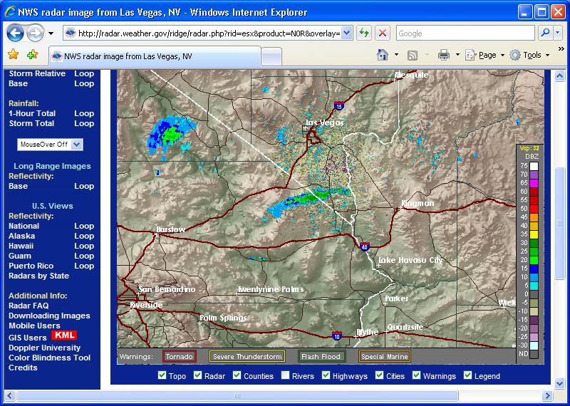
For example the radar site id is ESX and the DSID is 10215. The radar site id is displayed on the
radar image screen in the center of the radar site navigation arrows.
Boundary File Name Example:
NexradBoundaryESX10215.txt
Point File Name Example:
NexradPointESX10215.txt
These 2 files are placed in your Getrealtime file directory.
Once you have generated these two files then you have to add site information to
the GetAccess HDB database and to the GetRealtime setup file.
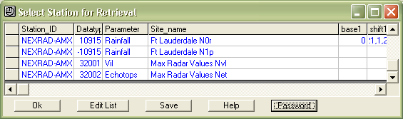
The Radar coefficients can now be checked and entered by using the 'Wizards' button on the Select Station List. Just
click on your station, if present, and then click 'Wizards'.
You will see a complete breakout of all your coefficients for editing.
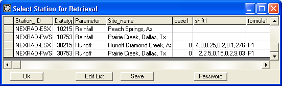
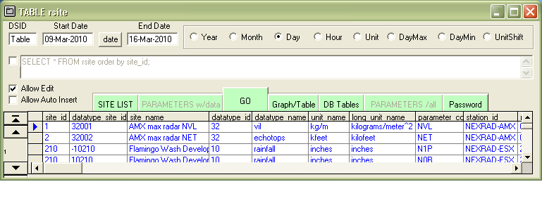
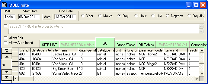
Here is an example of the data required in the GetAccess HDB table Rsite for
both runoff (30) and rainfall (10):
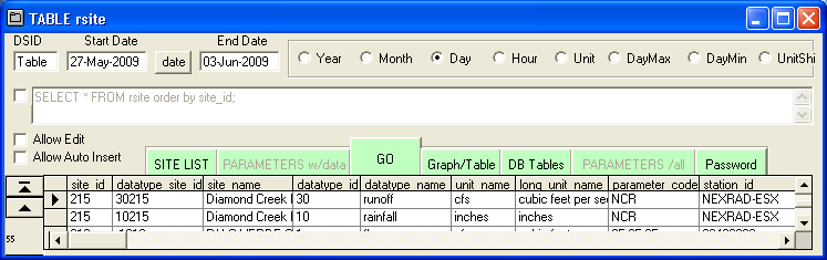
The new crucial information is in fields Parameter_Code and Station_ID. The Parameter code is the type of
radar image being used, either 1-Hour Total code=N1P, Base Reflectivity code=N0R or Composite
Reflectivity code=NCR. NCR seems to
be updated more consistently during storm events than N0R but I may be wrong.
1-Hour Total seems preferable anyway. And N0R is spelled with a zero.
I'm beginning to like the N0R more and more. I have only been at this for
a week.
The N1P 1-Hour Total radar images ARE NO LONGER treated differently than N0R and NCR
rates. If the GetAccess HDB database has accumulated more than 1 hour of unit values then
the interval rainfall amount is computed as
RadarNow-(RadarLag1-UnitValueLag60&Interval) else it is simply
RadarNow/(60/interval). I may be on a fool's errand trying to sample an
irregular radar time series at a regular interval with lag. We shall see.
Note: Getrealtime.exe 1.3.9 updated 12/18/09 now treats the N1P rainfall
1-Hour Total just like the N0R and NCR in/hr. It seems to make more sense, but
tends to lag the rainfall over the hour.
Although Storm Total NTP images would avoid potential error in lag of the 1-Hour
Total, their resolution seems to be too grossly graduated at the lower values to
be much use for farmers and fire hazards in the West and for runoff from small
basins, but I may be wrong again. I will add Storm Total soon for those living
in swamps and other backwaters so check back often.
Update 8/27/2016: Ridge2 5-minute product PTA storm total hase
been added to GetRealtime. The Rtable setup for parameter_code is 'PTA-Ridge2'. The
DataType_ID is 9 for total rainfall. It is interesting to compare with N0Q
hourly totals to see how it does but lots of early experience with the precip
product N1P was a complete dud. PTA uses the new QPE algo so it bares watching.
The boundary and point file are the same as N0Q so copy and rename the -10 to -9
part like this:
NexradBoundaryBGM-9301Q.txt
NEXRADPOINTBGM-9301Q.TXT
I have updated Getrealtime to let users put there own DBZs to rainfall rates in
the setup SHIFT cell like this:
NEXRAD-AMX; 10915; Rainfall; Ft Lauderdale N0r;
0; 0.00, 0.00,.02,.04,.09,.21,1,2,4
(don't forget that 0 goes in the BASE cell and the
first dbz=10 to change)
Note that not all the upper rates are needed if not revised. I have updated
GetNerad.exe (and GetRealtime.exe) to allow users to change the rainfall rates in the same manner by
including the optional file 'Dbz2Rainrate.txt' that has just the one line that
looks likes this:
0.00, 0.00,.02,.04,.09,.21,1,2,4,7,10,11,12,13,14
With the new Ridge 2 higher resolution products, look at the conversions in
the file 'Level2RGB.txt' for selecting or changing rainfall conversion rates.
More help examples are available at
http://getmyrealtime.com/RainfallComparisons.aspx and
http://getmyrealtime.com/SierraSnowfallComparisons.aspx.
The Station_ID in this example is NEXRAD-ESX which tells Getrealtime to use the
ESX site radar for imagery acquisition.
You might notice that new datatype_id that must be used for Runoff computation
is 30 and the datatype_id for rainfall is still the old 10.
Here is an example of the data required in the Getrealtime setup file
GetRealtime_setup.txt for both runoff (30) and rainfall (10):
Notice first that the Rainfall for a station is retrieved before the runoff can
be computed and so is placed before it in the setup file. Again the Station_ID in our example
is NEXRAD-ESX.
Or... version 2.0.1 can now use Station_ID= COMPUTE-Unit like
this:
COMPUTE-Unit; 30755; Runoff; Prairie Creek, Dallas, Tx; 0; 2,2.5,0.15,0.2,9.03;
P1
The HDB database table RSITE would have the Parameter_Code= 10753 and
Station_Id= COMPUTE.
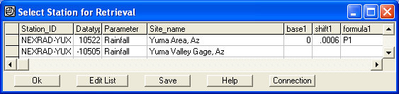
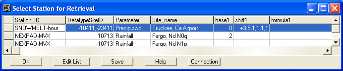
If your site of interest is too near the radar site and causes false background
readings then you can put a lower bound on the radar rainfall values being
recorded by entering a shift1 and formula like this:
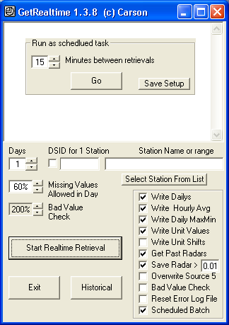
Images available for
the past 4 hours will be retrieved and processed (24 images in clear mode, 48
rain mode). The easiest batch mode method is to check the checkbox
‘Scheduled Batch’ and GetRealtime will go to sleep between retrievals. If
the batch interval is set to 5 minutes or more then up to all 4 hours of past radars will be retrieved on first
retrieval, then just the need latest images. Radar need not be retrieved
when there is no rainfall. Runoff computations will fill in zero rainfall for
missing periods of rainfall in the 5-minute record.
Does This Radar Stuff Really Work???
Let's compare with an actual point rainfall gage. (This better pan out well is all I know)
Example of how to create a Boundary File and a Point file for a 1-Point
Wunderground weather station comparison. As above, create a boundary file for a
very small area around the weather station location. Only the column of X,Y
pairs matters. From here knowing the center coordinates hand edit the XY
boundary by hand similar to this (any size is ok):
Edit boundary for a better square Area1 X,Y Coordinates (pix)
322, 188
322, 190
324, 190
324, 188
322, 188
Xmin 322, Ymin 188, Xmax 324, Ymax 190
Centroid= 323, 189
Now you can use Notepad to create this simple Point file:
323,189,323,189
1
That's it, just 2 lines. The reason for creating a larger area boundary file is
so you can see it on the computer screen and can click on the color within it.
The Point file does all the work.
The utility program LatLongPixels has been added to more accurately determine
the point file value needed given the points Lat/Long values. Wundergrounds
weather stations all have their Lat/Longs on their station location screen on
the right side of their current daily history pages (the pages with the 'comma
delimited download' option. You may download this utility
here.
I am using these 2 file examples for the Miami AMX radar to compare with the
Wunderground weather station KFLCORAL5 west of Fort Lauderdale, Florida. Why
this particular station? Because it was somewhat near a highway intersection for
locating on the radar image and appears to be well maintained. How would I know? Because I can read maps and also wind speed is a dead give away. The
least amount of calm is golden. But most of all, you want some rain to be
recorded when it is raining, duh. And the last thing, but minor, is time step. I
really like 10-minute and 5 minute time steps that appear regular but it's not
critical. Wunderground
stations can be jewels or really bad losers so check them out. I will try to
post some data on this Nexrad vs Wunderground example soon... if it works out
favorably, otherwise I'm burying it. ;-)
For the results of these rainfall comparisons go here.
For an example of how to automate GetRealtime Nexrad radar-runoff and the results of these rainfall-runoff comparisons go here.
GetRealtime 1.5 updated 1/2/2010 will route and combine runoff and
flow hydrograph values in the GetAccess database. To do this start with
GetAccess.exe, select DB Tables, Rsite, and add a new line like this:
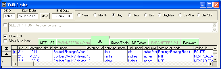
The new parameters are Parameter_code and Station_id.
Rsite table setup in GetAccessHDB.mdb Access database:
DSID=1xxx
DataType_ID=1
Datatype_name=flow,....
Parameter_code=FlamingoRoutingFile.txt <<< your routing control file name
Station_id=ROUTE
Now set up GetRealtime.exe's GetRealtime_setup.txt file like this:
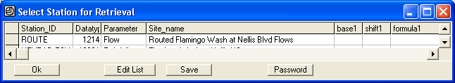
Station_ID; DatatypeSiteID; Parameter; Site_Name;
ROUTE; 1214; Flow; Routed Flamingo Wash at Nellis Blvd Flows
Some routings with
long travel times may need more than 1 day of warmup before writing the values to
the HDB. For longer warmup days add the days in base1 setup
field like this 7 days:
ROUTE; 1214; Flow; Routed Flamingo Wash at Nellis Blvd Flows; 7
Place the routing below any of the retrievals or runoff computations in the setup
that will be routed.
Input time-steps other than 5-minute, Route-xUnit can be used, ie. Route-10Unit
for 10-Minute Candian Radar runoff. Or Route-xHour or Route-xDay for hourly and
daily runoff.
Now all we need is to create the routing control file. The control file consists
of the 7 commands:
GET (gets flow values from GetAccess HDB database)
COMBINE (adds the current working hydrograph to the last combine
hydrograph)
SUBTRACT 0 or 1 (subtracts the current two hydrographs, a 1 value
reverses order)
ADD (adds a constant value or hourly to the current hydrograph, negative value for
loss, see release)
RELEASE (replaces outflow values less than release in modpul outflow
rating or ADD)
ROUTE (routes the current hydrograph using Tatum, Modpul, Muskingum, or
Muskingum-Cunge)
DIVERSION (diverts from the current hydrograph by using a diversion
rating and by providing a DSID you could later GET this diversion, route, and
combine.)
IF (set modpul rating based on dsid or date each day or skip-n
lines at start)
PUT (change output dsid)
WRITE (debug routing output file RouteSteps.txt)
END (end and write current hydrograph to HDB database)
As an example text file named FlamingoRoutingFile.txt:
Your
single Title Line Here is a must.
WRITE turn on debug file. Can be set anywhere
GET 4 30752 Upper sub Prairie Cr (30752 is the
DatatypeSite_ID for Sub Prairie Cr)
GET 4 30753 Lower sub Prairie Cr (4 indicates unit values,
3=hour, 2=day, GetRealtime_setup overrides)
COMBINE
ROUTE Tatum 2.5 travel time in hours
ADD -2.5 reduce all the current hydrograph's values
by 2.5 cfs
GET 4 1754 Trib sub dallas river
COMBINE
ROUTE Muskingum 2.0 0.25
3 lag in hours=2 and X=.25 in
who knows, cascades=3.
ROUTE Muskingum-Cunge MCungeBeaverCr.RAT
GET 4 1758 Little sub trib
COMBINE
DIVERSION 1888 CulvertDiversionAt56thSt.RAT
dsid=1888, use dsid=0 to not save diversion
GET 4 1757 Left fork sub trib
COMBINE
RELEASE 12000 schedule 12000 cfs constant release
from Lake Mead modpul rating
ROUTE Modpul
3777 LakeMead.Rat you can add optional DSID for
writing elevations and startup flow will use this elevation so always use for
reservoirs.
RELEASE -1404 -1 get release from
rhour dsid hourly
ROUTE Modpul
Steephill.Rat 3 Steephill.Rat 3 a 2 or more for cascading Modpul
or 0.01 to 1.99 for storage adjust
IF 0 rday PARAM SteephillOCT.Rat month(D)>9 (no comments allowed)
ROUTE Modpul
Steephill.Rat -1 a -1 will use the optimal N
cascades from Modpul 4th column
ROUTE Modpul
3777 Steephill.Rat -2 0.75 a -2 will include daily Seldon
KS evap*0.75
ROUTE Modpul 3777 Steephill.Rat -3 0.75 a -3 will include
daily Seldon KS evap*0.75 AND start on actual starting day, not at beginning of
runoff. Use this if you have actual elevation history.
RELEASE -1401 -1
RDAY get release dsid hourly and yesterday mean for projected
ADD -1
remove release value times -1, use +1 to add
PUT -1102 change output dsid, may be needed for
overwriting USGS gage
END
(Any notes after the END command will be ignored)
Note that after the initial two GET's, there after, every GET a COMBINE must
follow at some point. To make your routing easier to follow, try to combine as
soon as possible. For instance you cannot be routing two streams at the same
time so use COMBINE first. The current or working hydrograph to which
ROUTE, ADD, and DIVERSION are applied is determined by the last COMBINE or
last GET, which ever was last.
Also note that while GetRealtime is running in Batch Mode, unlike the
GetRealtime_setup.txt file values, any changes made to the routing files will
take affect on the next run. So using the Routing Wizard you could
change Releases, Adds, and such in the routing files with out restarting
GetRealtime.
Update 6/21/2016: If you have a reservoir in your basin like a
USBR Pacific Northwest dam with near real-time lake levels and river and canal
releases info then you can use a MODPUL routing with out resorting to shelling a
reservoir model like Hec-RESSIM. This allows forecasting the next 7 days of
river/spillway releases with the NWS forecast for runoff with just a simple
Modpul. Also note a reservoir rule curve is just another Modpul rating and
can be used per Date with an IF check .
EXAMPLE Modpul Routing File:
Route Subs 8,9,10 runoff thru Emigrant Dam
GET 4 -1108 Subs 8-9-10 inflow
RELEASE -25401 -1 RDAY get each hour but yesterday mean for projected
ROUTE Modpul 3401 EmigrantDam.RAT overwrite Hydromet elevs in 3401
RELEASE 25401 -1 use Hydromet canal hourly
and last hourly for projected
ADD -1 use release *-1 to remove canal for river release
END
The
hourly 'RELEASE' can be used by both 'MODPUL' and 'ADD'. You could also hand
enter hourlys in rhour values in rhour table to schedule RELEASE values
manually. When you write '3401' Modpul elevations, then GetRealtime knows to get
starting elevation from database. Note small reservoirs without release
info can use MODPUL just as well without RELEASE with a wel thought out Modpul
rating and is how normally used.
EXAMPLE
Lagged Release to use last weeks values hourly or dailys for projected:
Subs 8+9+10 as combined inflow into Emigrant Dam
WRITE
GET 4 -30109 Sub 9
RELEASE 1403 -1 RHOUR-7 Green Springs
Powerplant bottom Sub 9
ADD +1 add
RELEASE 1405 -1 RDAY-7 West Side Canal
ADD -1 remove
GET 4 -30108 Sub 8
COMBINE GET 4 -30110 Sub 10
COMBINE
END
The 'IF' can be used with 'MODPUL' to set the rating file name each day like
this:
Route Subs 8,9,10 thru Emigrant Dam
GET 4 -1108 Subs 8-9-10
RELEASE -25401 -1 use Hydromet hourly value for today and projections
IF 0 rday PARAM EmigrantDamJAN.RAT month(D)=1
IF 0 rday PARAM EmigrantDamFEB.RAT month(D)=2
IF 0 rday PARAM EmigrantDamOCT.RAT month(D)>9 and month(D)<=12
ROUTE Modpul 3401 EmigrantDam.RAT use defualt Rat if not triggered above
IF -30103 rday SKIP-1 flow P1>10
ADD 5
END
All routings start a day early for warm up before writing the requested start
date values so something to be aware of.
Update 7/7/2014: Muskingum routings can use cascades
by just adding the number of cascades as shown above. The wedge storage X
factor can vary from 0.5 for no storage to negative values. Start with X=0.2 and
if cascading try some negative X values. Cascades have the effect of
non-linear Muskingum coefficients,
so they say, and
much easier to calibrate. My free ModPulXsec.exe on my More Stuff page can
compute the Muskingum-Cunge K & X and number of cascades using the SCS
TR-20 methods for constant
parameters based on peak flow. The Muskingum-Cunge rating file produced by
my ModPulXsec.exe shows the format for using a constant parameter
Muskingum-Cunge routing based on the peak flow look up.
GetRealtime 2.4.0 Modpul routing can now perform a
cascading subdivision of your rating by dividing your rating
storage values by the number of sub-divisions and then loop the routings. This
has the effect of increasing peak outflow as N increases. To perform a Modpul
sub-division, just enter a 2 or greater value after the rating filename as shown
above. For more background on cascading Modpul and other routings read
Heatherman's pdf info here. (Another tip of the hat to David in Alabama.)
Also a Modpul cascading subdivision value entered between 0.01 to 1.99 will be
used not as a subdivision but as a modpul storage
adjustment factor. Example, if 0.6 is entered then the modpul rating
storage values will be multiplied by 0.6. This makes calibrating routings much
easier and may be just what you needed all along instead of cascading for a
larger peak. I wonder if they ever thought of that?
To calculate the number of cascading reservoirs to match a full unsteady flow
solution, the pdf author says:
N=(W*L/K)*Z/Q =number of cascading reservoirs
where:
W=cross-section top width, ft
L=entire reach length,ft
K=travel
time as dVol / dQ, seconds
Z=fall over the reach, ft
Q=flow, cfs
Use Hec-Ras or my free ModPulXsec.exe to compute these factors at a typical
cross-section.
Ideally you would select a flow at 2/3 the peak inflow hydrograph, but I guess a
Modpul-Heatherman could make this adjustment on the fly for each Modpul file
line: elev, flow, storage, N.
Update Nov 18, 2013--I have added the optimal N number of cascading reservoirs
to my free ModPulXsec.exe (see More Stuff page). Now if you add a -1 for the
number of cascading reservoirs Modpul will now get the 2/3 of the inflow peak
and lookup the optimal number N reservoirs:
ROUTE Modpul
Steephill.Rat -1 a -1 will use the optimal N
cascades from Modpul 4th column
ROUTE Modpul
Steephill.Rat -1 0.5 with a 0.5 peak lookup
adjustment
if the 0.5 is included then instead of 2/3 peak flow lookup a 0.5 peak flow will
be looked up for optimized N.
Muskingum K=3.0, X=0.3, cascades=12:
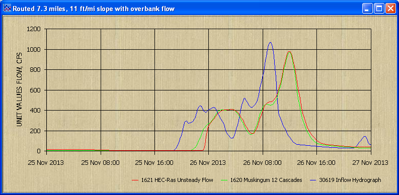
Muskingum with cascades can be nearly as good as Modpul, but for the number of
optimized cascades you will still need to figure that out. I just used the
Modpul's optimized number from its average cross-section computations. The
advantage of Modpul then, is you do not need to know K travel time or X storage
factor, but if you have an outflow hydrograph then these are easily fitted. Or
even if not, my free ModPulXsec.exe computations can give the constant parameter
Muskingum-Cunge estimates. Better to estimate a cross-section and use Hec-Ras
unsteady flow routing with interpolated x-secs and see where your Modpul or
Muskingum should be heading and if it won't work then automate Hec-Ras unsteady
flow to do your routings for these difficult reaches.
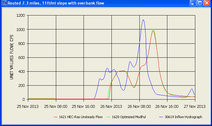
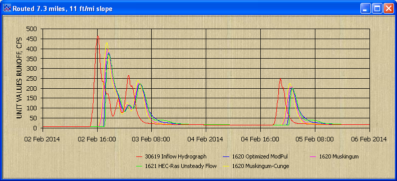
Below are comparisons with Muskingum-Cunge calculated K, X, and cascades.
I have found HEC-Ras unsteady cannot route a mountainous 55 ft/mile slope
channel but both ModPul and Muskingum seem to do fine.
The 'RELEASE' command will replace the next modpul outflow rating values above 0
(0 is needed) with the Release value if less than the release. This will produce
a constant release until storage is above this value or empty. The Release
command allows an easier change in schedule than redoing the whole modpul rating.
The 'Release' command can also preceed an 'ADD' command as shown above. The Routing Wizard will allow easy access to the routing files for easier
changes like this.
If your basin has more than one main channel, then you will need to write a
separate control file for it and save each channel in the HDB database before
combining with the last control file. Remember to try using my
ChannelStorage.exe
(trapezoidal) or ModPulXsec.exe (x-section) available
here to create the Modified Puls channel rating or velocities for Tatum and
Muskingum peak travel times.
ModPuls Rating example:
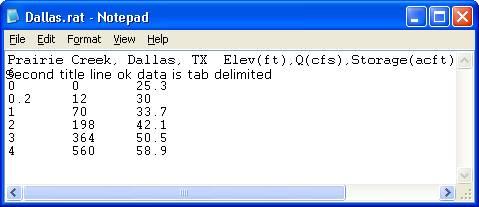
Diversion Rating example of 2 columns for Qin and Qout where Qin is flow in the
channel at the diversion point and Qout is the diversion:
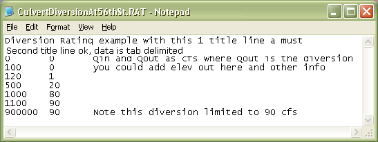
The diversion record can be saved with a DSID and then returned using MODPUL
rating or some math function based on other parameters. Not sure how you would
do this so you might think about it.
Update 1/18/2014--To change a 15-minute USGS flow time step to 5-minute steps
add ', 5-min' on to the USGS station number on the GetRealtime_setup.txt:
094196781, 5-min; 1211; Flow; Flamingo Wash at Nellis Blvd
This allows adding a forecast to the USGS gage which the USGS gage can overwrite
as the observed data becomes available. Why?... because now you can route and
combine gaged flows with other sites 5-minute time-steps.
Update 12/18/2013: Runoff computations done with datatype_id=30 when run by the
number of past days now checks for a recession runoff on or
after the start of computations and if it is then the starting day is moved to
the day of the starting runoff plus 1 day. This insures you are not cutting off
a previous recession. The start and end of runoff are now stored in the table
'rupdate'. The earliest starting day for the run is then used for all subsequent
routings including the HEC-Ras and HEC-Hms shell routings. Runoff computed by historical
dates do not store anything in the table 'rupdate' and do not self adjust
starting date.
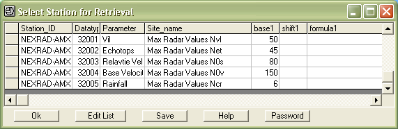
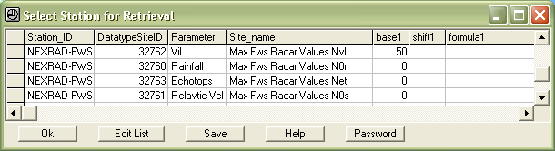
GetRealtime 1.5.1 updated 3/18/2010 now supports NEXRAD Radar
images for NVL (vertical integrated liquid), NET (echo tops), N0S (storm
relative velocity) and N0V (base velocity) as well as the N0R, NCR, and NTP
rainfall conversions for the scientifically minded. Although a screen area
averaged NVL and NET make little sense, the maximum value on the radar screen
can be used as an early warning for hail storms and other exciting things. To
determine the maximum value on the Nexrad radar image a new Datatype_ID has
been added and is 32 to indicate a radar image maximum is wanted. See list of
Datatype_ID's above. Remember valid SDID integers are -32,768 to 32,767 so your
Site_ID is limited to 1 to 767 instead of 1 to 999.
Use GetAccess to set the HDB rsite table as follows:
Now add the site to GetRealtime_setup.txt using either Notepad or
GetRealtime.exe itself like this:
Now we need a Boundary file to determine what points will be checked on
the radar image. The boundary needs to cover the 143 mile radius around the
radar site and so using Notepad the Boundary file will be a rectangle like this
named NexradBoundaryAMX32001.txt:
Miami AMX Full Radar Area
10,15
10,534
589,534
589,15
10,15
Xmin 10, Ymin 15, Xmax 589, Ymax 534
Centroid= 299,274
Note that Ymin and Ymax can be shrunk at higher latitudes and you can trim some
fat off the rectangle by adding 0.292 and 0.708 of the height and width for an
octagon like this:
Miami Full Radar Octagonal Area
10,167
10,383
179,534
420,534
589,383
589,167
420,15
179,15
10,167
Xmin 10, Ymin 15, Xmax 589, Ymax 534
Centroid= 299,274
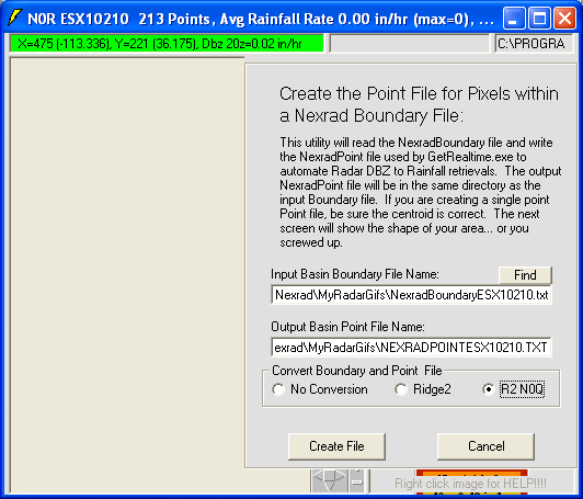
Lastly all that is needed is the Point file. The Point file is
created using GetNexrad.exe. Fire up GetNexrad.exe and select 'Create Point
File' and select the Boundary file name located in the GetRealtime folder above
like this:
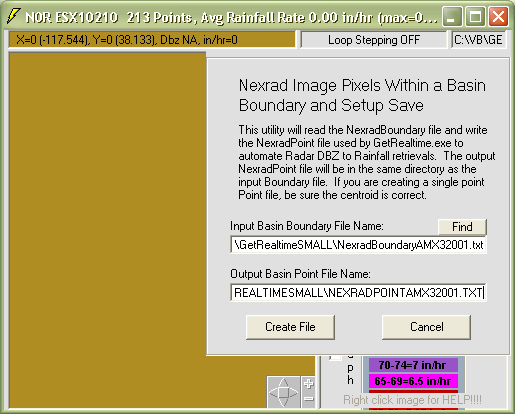
Select 'Create File' and answer 'NO' when prompted 'Do you want to create a
single point file?'.
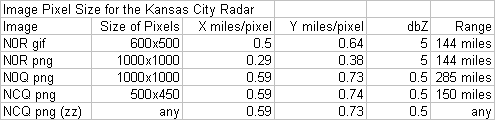
The 580 x 450 boundary will contain 261,000 points in the point file. Luckily
the pixel size for the radar NET and NVL data points is about 5 pixels by 5
pixels for the 2.5 x 2.5 mile coverage so only every 4th pixel needs to be
checked reducing the actual work to 16,312 pixels... child's play. On the other
hand if you want the maximum for a NCR image all 261,000 pixels will be
checked... ouch!
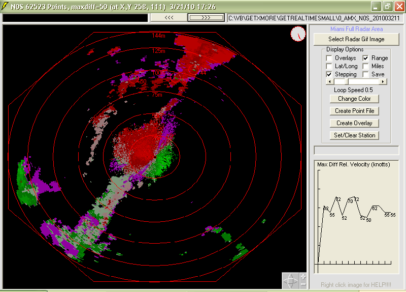
The maximum N0S and N0V velocities are checked every other pixel or about 1 mile
apart. The storm relative velocity maximum difference is calculated as the
difference between non-zero values of opposite signs (-inbound and +outbound
velocities) and can exceed the max 50 knots and 99 knots. Nearly all N0S images plain maximum
velocity are near the maximum value of 50 knots and so is of little use hence
the difference calculation. Green next to Red, means your dead... or its
birds and bats and business as usual... boy those guys at headquarters keep us hoppin.
We are all set to automate GetRealtime in batch mode as discussed above. You may
wish to save radar gif images with maximum values above a certain value by
checking the Save Radar box and be alerted by a beep by checking the Beep box. I
normally run GetRealtime in batch mode like this:
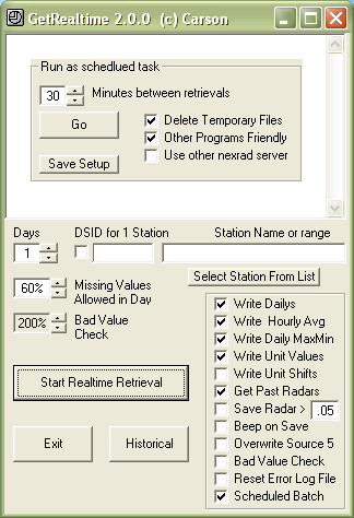
The 'Delete Temporary Files' when checked will delete temporary internet files
and history that Internet Explorer saves in it's temporary files location, BUT
NOT any gif image files you wanted saved in the normal download location.
Normally it is best to check this box.
If a Gif file download is timed out, GetRealtime will try to down load the gif
again before moving on.
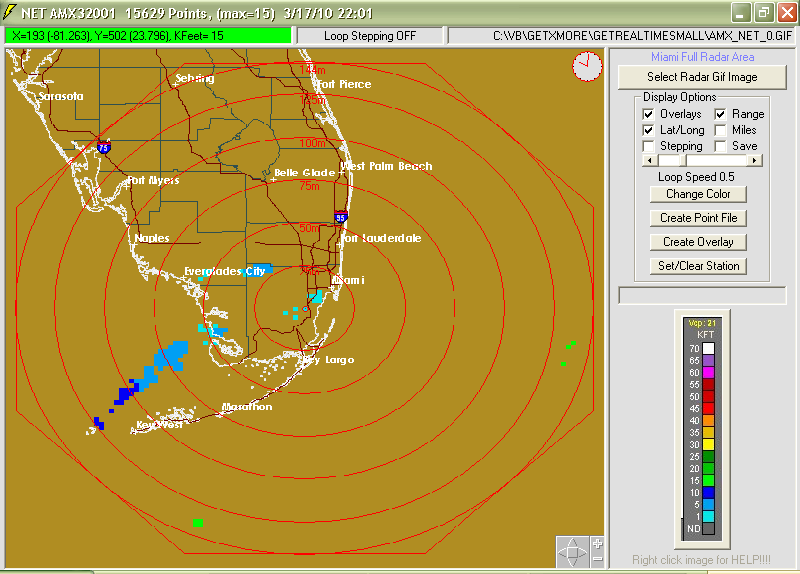
Below is an Echo Tops NET radar image as shown by GetNexrad and the octagonal
area maximum value 15 is shown in the window caption as well as the point I
clicked on:
Here is an N0S max velocity diff example:
Radar gif images may be saved to file when values exceed the value entered in
the 'Base' field as shown below and will over ride the value entered on the
GetRealtime main screen when 'Save Radar' is checked. If the base value is below
0.01 it will be used to remove rainfall values that are caused by ground clutter
as described above. Ground clutter is removed on the NCQ and A2M radar images
for you.
If you would like to save all the 32 datatype radar images at a site based on
the first of a series being saved then enter '0' as 'base1' for the subsequent
like this:
Note: NET and NVL have been discontinued.... "As
part of troubleshooting some RIDGE delivery problems, we discontinued these two
products as part of troubleshooting. The products will restart when RIDGE2,
version2 is deployed. This is not likely until after the start of 2012." ~NWS
ROC~ ...but are currently available on the Ridge2 Testbed below.
RIDGE 2 TESTBED
GetRealtime.exe has been updated to read the new 1000x1000 pixel PNG files
available on the Ridge 2 Testbed. The new higher resolution DBZ
product N0Q has 0.5 dbz resolution compared to the old 5 dbz resolution and
should be your base reflectivity product of choice.
New GetNexrad 3.6.0--Iowa State
University Mesonet historical images can now be directly loaded for a
loop of up to the past 24 hours for Ridge2. Historical radar images
beginning Jan 1, 2012 can be downloaded for 24 hours, 1 day at a time.
Images download at about 6 hours per minute.
Update 12/9/2014: I added a 'Max radar hours' to the GetRealtime.exe batch menu.
If you haven't run the radar in a few days it will get up to the past X hours of
radar. So if you run your radar once a day and want ALL THE RADAR since
yesterday, set the 'Max radar hours' to 48. It will get all the radars since the
last time it ran yesterday. I wouldn't recommend getting all the radars but you
could. And you don't have to actually run in Batch mode. Just check the Batch
box, set the max hours, then UNcheck the Batch Box and run. And apparently Iowa
now allows at least 48 hours per download. I just tried it. So don't think you
have to run GetRealtime exactly at the same time each day. Even if Iowa goes
back to a 24 hour limit, then run it twice a day. But I wouldn't. This will come
in handy if you know it started raining some time last night. You could use
History but History doesn't set the last radar retrieved time.
Your old boundary files can be upgraded to the new Ridge2 world files using
GetNexrad.exe and is as simple as choosing the short range or long range N0Q
product. Although as of 8/8/2012 GetNexrad no longer needs to covert
boundary's between Ridge 1 and Ridge 2 and KMZ, GetRealtime must use Ridge
version specific boundaries. All GiF images are Ridge 1 and all PNG images are
Ridge 2. The conversion here is only one way from Ridge 1 to Ridge 2.
With the new N0Q 0.5 dbz resolution, the
new file "Level2RGB.txt" allows on the fly
choice of rain rate type conversion such as Convective 0, CoolWest 1, CoolEast 2,
Tropical 3 and Semi-Tropical 4. To tell GetRealtime which rain rate conversion type
to use simply put a 0, 1, 2, 3, or 4 in the GetRealtime setup file Base1 setup
cell or leave blank for Convective.
In the GetAccess Database the new Parameter Code is the product code with
"-Ridge2" attached like N0Q-Ridge2.
Remember Ridge2 is a Testbed and may change so if problems
occur check back for updates to GetRealtime.exe.
For much more info on the Ridge2 products, see the
GetNexrad Help web page.
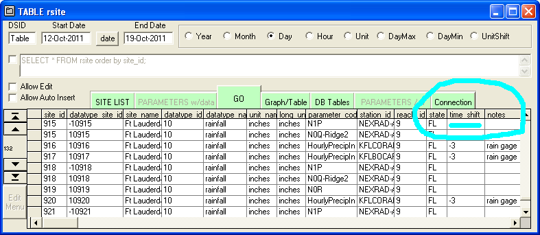
Shifting Retrieved Times to Your Time Zone
Update 10/19/2011 allows GetRealtime retrievals to be adjust for any time value
or time zone. The GetAccess 'rsite' table now has a field 'time_shift' which you
can enter the hour shift. To adjust a Wunderground station in Florida (ET) to
your home in California (PT) then you could enter a -3 for the 3 hour time zone
difference in table rsite field 11 ('time_shift'). This makes comparing Nexrad radar stored in your time zone easier.
If you add this field 11 to your database table 'rsite' it is a double precision
floating point.
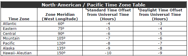
One caveat to this is computations of Solar and ET is when you are using
COMPUTE instead of the Station_ID. You then need to use
your standard time meridian, which is 15 degrees per hour. Central to my
Pacific time would change solar noon from -90 to -120 for the 2 hour diff so you
have to fix your GetRealtime_setup if you use the COMPUTE method.
Daylight Savings Time change is ignored. Spring forward will leave an empty hour
between 1 am to 2 am and Fall back will over write the 1 am to 2 am unit values.
Hey, you voted for these knuckle heads.

Snowpack and Snow Melt
Update Dec 2, 2020: I have added downloading modeled snow data
from NOAA's National Operational Hydrologic Remote Sensing Center's Interactive
Snow Information (see below):
https://www.nohrsc.noaa.gov/interactive/html/map.html
Ive also started a comparison of GetRealtime's snowmelt with adjusted radar to
the NOAA Snowcast modeled data here:
http://getmyrealtime.com/SnowmeltComparisons.aspx
(Update 12/3/2011)
GetRealtime.exe
2.2.1 has been updated to compute a continuous year around simulation
of a point snowpack accumulation and melt. The melt (output as a rainfall
parameter) can be input to
Getrealtime's rainfall-runoff for a real-time continuous simulation through out the year.
And yes, the snowmelt calculation will give the correct precip even in July...
in Death Valley.
GetRealtime has adapted the methods of the physically based point snow surface
hourly
model
ESCIMO (Energy balance Snow Cover Integrated MOdel) (Strasser et al., 2002)
for hourly, 5-minute, or daily time steps for simulation of the energy balance, the water
equivalent and melt rates of a snow cover. ESCIMO uses a 1-D, one-layer process
model which assumes the snow cover to be a single and homogeneous pack, and
which solves the energy and mass balance equations for the snow surface by
applying simple parameterizations of the relevant processes... like I would
know.... it's just science.
Update 9/20/2012--The Snowmelt coefficients can now be checked and entered
by using the 'Wizards' button on the Select Station List. Just
click on your station, if present, and then click 'Wizards'.
You will see a complete breakout of all your coefficients for editing.
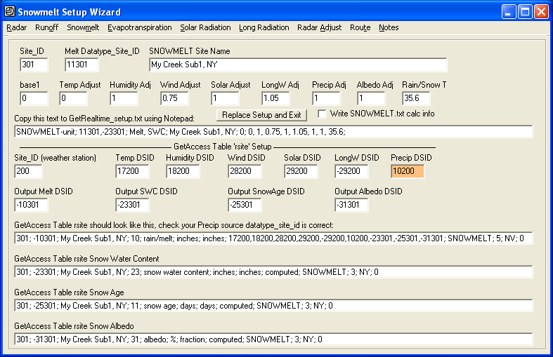
Example GetAccess 'rsite' table for snowpack:
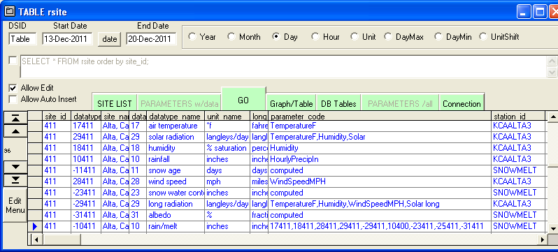
The station_id SNOWMELT parameter_codes order must be strictly followed but the
site_id part of these datatype_site_id's are up to you. I would assume you would
want to use a Wunderground gage for these first five inputs but compute the
output for another site_id meaning the last four datatype_id 's 10, 23, 25,
and 31 can
belong to your real point of interest. This example computes the snowpack for
the Wundergage site but with Nexrad Radar precip so has a different input precip
site_id.
In the station_id SNOWMELT output precip datatype_id code is 10
for rainfall, which I named rain/melt here and has the parameter_codes:
17411,18411,28411,29411,-29411,10400,-23411,-25411,-31411
Temp. 17
.....,Humidity 18
...........,Windspeed 28
.................,SolarRadiation 29
.......................,LongRadiation -29
..............................,Precip Input 10 (the
output Rain/Melt is this whole rsite record)
....................................,Output SnowWaterContent
-23
...........................................,Output SnowAge -25
..................................................,Output
Albedo -31
Albedo output has been added because the starting value really cannot be
calculated from just Snow Age because of it's variable recession coefficient
history. And as it turns out, it seems pretty important so needs looked after.
Example GetRealtime_setup.txt:
Station_ID = Snowmelt-hour or Snowmelt-unit (yes, 5-minute snowmelt!)
The shift1 cell is used if you would like to adjust the 6 input parameters above
and the 7th adjustment is for Albedo decay rate (<1 to slow down ripening but
this decay factor * (-0.12 or -0.05 ) only applies if snow age is greater than 7
days). You may leave shift1 blank or just add up through your parameter of
interest. For example to add 3.5 degrees F to the Wunderground input only for a
different elevation of interest, then only the first +3.5 is needed. I'm really
not sure how one would adjust say Solar radiation for north or south exposure
but you can change the multiplicative factor 1 here following the strict
parameter order above like +3.5, 1, 1, 0.8, 1, 2.1, 1, 35.6
The ending 35.6 is the rain/snow temperature F
phase which corresponds to 2 degrees
kelvin above freezing. When kicking off a season with warm soil you may
want to lower this to 32F or even lower to get runoff.
Air temperature determines if the precip is snow or rain and is also used in the
heat transfer calculations and so it is probably a good candidate for first
adjustments... then probably longwave radiation. The albedo can be adjusted
after 7 days for
swiftness of the spring melt on larger snowpacks or slow down long winter dry spells.
When there is snow on the ground, runoff losses are reduced 15% to simulate
frozen soil.
On 2nd thought, if you change any of the first 3 (Temp, Humidity, Wind) for use
at your real site of interest, then you will need to recompute Solar and
Longwave Radiation, which can be done, but I need to make a Temperature change as
painless as possible.
Based on my regression formula at this elevation, a 3.5 F Temperature change
would cause a 3.4% change in Longwave Radiation over the year or about 1% for
each degree F. This probably means that a 1000 ft elevation lapse rate of
-3.5 F change should be nothing to worry about for radiation. I already have
found the Longwave Radiation factor needs to be less than 0.5 in the Sierras to
keep the current snowpack from completely melting. (not to worry, see
graph below)
Update: I suggest Shift1 as: 0, 1, 1.15, 1, 1, 1, 1,
34
Based on NWS Snowcast info and modeled runoff at
several sites around the US. The 1.15 windspeed adjust is an assumed 12' height
gage corrected to 30'. The melt calculations use 1/10 this speed. Wind is
important because of the large sensible heat flux it figures into.
Changing the input Precip is ok, ie., 2.0 for 2.0 times the N0Q radar precip at
your site or drainage area of interest. And if you add a '0' after the
rain/snow 35.6 factor then the computation steps will be printed to the file
'SNOWMELT.txt' which you can paste/open with Excel to read. After the novelty
wares off, remember to delete the 0.
Input Example GetRealtime_setup.txt:
KTRK; 17411; Temperature; Truckee, Ca Airport
KTRK; 18411; Humidity; Truckee, Ca Airport
KTRK; 28411; Wind Speed; Truckee, Ca Airport
KTRK; 29411; Solar Radiation; Truckee, Ca Airport; 0; 39.320,-120.140,-120,5900;
P3 (*computed*)
KTRK; -29411; Long Radiation; Truckee, Ca Airport;
0; -4.55
(*computed -4.55F temp adj optional*)
KTRK; 10411; Precip; Truckee, Ca Airport
(Output)
SNOWMELT-hour; -10411,-23411; Precip,swc; Truckee, Ca Airport; 0; +0,1,1,1,1,1,1,33;
(note snow age datatype_id 25 and albedo 31 are also input/outputs as is snow water content 23 for
start up. Update 12/21/2012: If you run out of datatype_id 10 for
precip/melt then you can now use datatype_id 11 interchangeably with 10.)
When using snowmelt for GetRealtime runoff computation, the presence of snow
will be flagged (source 112 instead of 12) and runoff computation will reduce
melt infiltration by 30% (0.7 Snowmelt Loss Factor) for frozen soil. Also, ET will be set to zero. For your
spring melt runoff computation you could also MANUALLY set your
'Groundwater Loss Factor' to zero and its 'Groundwater Recovery
Adj' to 3 or so. Remember to reset these later to summer conditions.
One thing to note is that unlike I would have thought, it is not sunshine that
melts shiny new snow so much as the longwave infrared temperature of the
clouds and humidity and what ever else is up there... those heat fluxes...
beyond the horizon of perception. Ok, that is a lot of scientific
propaganda, everyone knows snow melts in the day. ;-)
Some tips on Long Radiation: The termperature lapse rate is 3.5
F per 1000 feet. Now you could for example compute each 1000 ft snowmelt band
long radiation with a temp adjust like shown above. Or you can compute the long
radiation at the weather gage and use a snowmelt long radiation adjustment
factor of 3% per 3.5 F or 1000 feet. The 3% comes from GetRealtime's regression
on the Escimo long radiation data using T, H, and Wind Speed and it has a
standard error of 24 watts/m^2: You could use a setup to compute your own long
radiation like this guy's:
"Parameterizastion of incoming longwave radiation in high-mountain enviroments"
L=5.67E-8*(T-21)^4+.84*H-57 ; where T= Kelvin and H= % Relative Humidity On my
Escimo radiation gage winter record this has a standard error of 31 watts/m^2
and I had to change the constant -57 to -20. I then get similar results either
method NWS 7-day forecast now includes 'cloud-amount' data_type 26 and
should be added to the parameter codes (see above computations)..
If you have used GetNexrad to enter multiple 6 or 24 hour QPF forecasts
then yesterday through today's rtable weather values will be used as needed for
snowmelt.
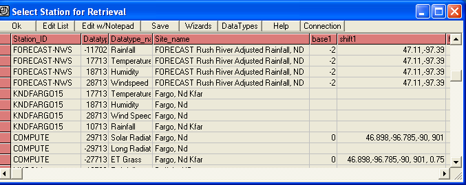
Update 12-23-2013: Better than using GetNexrad for snowmelt, GetRealtime will
now retrieve the NWS forecast for precip, temp, humidity, windspeed and
cloud cover
for the next 7 days for a lat,long. Because these values are not being
retrieved with the Wundergage site code you will have to change the GetAccess
table 'rsite' to use DSID's for computations of solar, long, and ET. Just
replace the Wunder Codes with the DSID's in the proper order. Also, like runoff
computations, snowmelt will then run up to the 7 additional future days
when run
by number of days. This is really slick, automated forecast of snowpack and melt
for 7 days! Here is a GetRealtime_Setup.txt example (The -2 is my time shift from
Central to Pacific):
If you are wondering why the redundant time shift in the setup file, you are
right about temp, humidity, and windspeed having the time shift in table 'rsite'
already but note my precip is a computed gage adjusted radar and
computed values will not or better not have a time shift in table 'rsite'. Also
see the 'Shifting Time Zones' caveat just above. The Solar and ET setup now
needs to use your standard time meridian.
Using Unit Values:
SNOWMELT-unit
When using Nexrad Radar 5-minute values only the period for actual precipitation
is needed. You do not need to keep the radar record going all the time.
When the Nexrad 5-minute values are present the weather gage input Temp,
Humidity, Wind, Solar, and Longwave are used at 5 minute time steps and output
will be 5 minute time steps. When Nexrad 5-minute values are missing, zero
precip is assumed and the output unit value time step will be the erratic time
steps of the Wunderground gage inputs. Add a zero to the 8th shift1 cell factors
as described above to see the full computations output for how this works.
Using Day Values:
SNOWMELT-day
Daily's seem to work also. You may want to investigate any changes to factor
adjustments that would be needed if any.
Using Elevation Bands:
In mountainous basins you can use Google Earth to see what fraction of your
subbasin is in elevation zones and compute each zone separately and sum like
this (notice ONLY the elevation band AREA is changed in the runoff coefficients):
******; *******; *******; ********Elev Bands*************
SNOWMELT-unit; 11492,-23492; Melt, Swc; 4000FT Burro Cr Sub 2 Snow Melt & Pack,
AZ; 0; 3.5, 1, 0.75, 1, 0.9, 1, 1, 34
SNOWMELT-unit; 11592,-23592; Melt, Swc; 5000FT Burro Cr Sub 2 Snow Melt & Pack,
AZ; 0; 0, 1, 0.75, 1, 0.9, 1, 1, 34
SNOWMELT-unit; 11692,-23692; Melt, Swc; 6000FT Burro Cr Sub 2 Snow Melt & Pack,
AZ; 0; -3.5, 1, 0.75, 1, 0.9, 1, 1, 34
******; *******; *******; *********Runoff Bands************
COMPUTE-unit; -30492; Runoff; 4000FT Burro Creek Sub2 Esx; 0; 3.18, 50, 0.1,
0.01, 39.672, 1, 0.1, 0.3, 3, 0.3, 6, 85, 50, 0.99, 0.7, 5, 0.7, 0.1, 0.05,
1.00, 0, 0.1, 1, 0.7, 0, LagV; P1; 0; Triangle Unit Graph
COMPUTE-unit; -30592; Runoff; 5000FT Burro Creek Sub2 Esx; 0; 3.18, 50, 0.1,
0.01, 98.154, 1, 0.1, 0.3, 3, 0.3, 6, 85, 50, 0.99, 0.7, 5, 0.7, 0.1, 0.05,
1.00, 0, 0.1, 1, 0.7, 0, LagV; P1; 0; Triangle Unit Graph
COMPUTE-unit; -30692; Runoff; 6000FT Burro Creek Sub2 Esx; 0; 3.18, 50, 0.1,
0.01, 33.174, 1, 0.1, 0.3, 3, 0.3, 6, 85, 50, 0.99, 0.7, 5, 0.7, 0.1, 0.05,
1.00, 0, 0.1, 1, 0.7, 0, LagV; P1; 0; Triangle Unit Graph
COMPUTE-unit; -30362; Runoff; Burro Creek Sub2 Esx; 0; 0; P1+P2+P3
Parameter values and constants used (updated 12-3-2011):
Parameter/constant Symbol Value Unit
Soil heat flux B 2.0 Wm−2
Minimum albedo amin 0.50
Maximum albedo (amin+aadd) 0.90
Recession factor (T
> 273.16 K) k -0.12
(32.0 F)
Recession factor (T < 273.16 K) k -0.05
Threshold snowfall for albedo reset 0.5 mm running sum for a day (0.02")
Threshold temperature for precipitation phase detection Tw 275.16 K
(35.6 F)
Emissivity of snow 0.99
Specific heat of snow (at 0 C) css 2.10×10³ J kg−1 K−1
Specific heat of water (at 5 C) csw 4.20×10³ J kg−1 K−1
Melting heat of ice ci 3.337×10⁵ J kg−1
Sublimation/resublimation heat of snow (at –5 C) ls 2.8355×10⁶ J kg−1
Stefan-Boltzmann constant 5.67×10⁻⁸ Wm−2 K−4
and... just so you know I know, 1W/m-2 =2.065 Langleys/day... geez I hope.
Also see my ongoing snowfall
study at:
Nexrad Snowfall Comparisons in western
central Sierras, CA
NWS Snow Model SWE and Melt, Depth, Temp, Snowfall & Rainfall
You can download HOURLY SWE and Melt forecast data of NOAA National Operational
Hydrologic Remote Sensing Center national (and southern Canada) snow model. You
determine a gage point (MADIS, CoCoRa, Lat/Longs, etc) and that's all you need.
You can use this interactive map to somehow find available Snow Model station
ID's. Turn off/on Stations and Cities and their Label to find your way around:
https://www.nohrsc.noaa.gov/interactive/html/map.html
Then you can enter your Station SHEF ID in the upper
right box here to verify data
is available (no snow cover will look like no data):
https://www.nohrsc.noaa.gov/interactive/html/graph.html?units=0®ion=us&station=CAN-ON-510
I'm not sure how one would use the Melt info in a runoff model. Does it include current rainfall or
not. I'm going on the assumption that if there is SWE values then rainfall is
ignored, if not use your supplied rainfall... but I'm guessing. Date_times are
adjusted to your PC's time zone.
Your GetRealtime_setup.txt would look like this:
SNOWCAST-NWS,CAN-ON-510; 11450, 23450; Forecast Melt, SWE; Ontario, CA
Where 'CAN-ON-510' is the 'Station SHEF ID' for data model point.
For table 'Rsite' you can use any of your other rain/melt and SWE DSID's or you
can add new ones. There is nothing used from table 'Rsite' other than the DSID's
and unit_names for Melt=11450 and SWE=23450.
Table 'Rsite' setup:
361; 11450; Snow Point Ontario, CA; 11; melt; inches; inches; xxxxxxx; xxxxxxx;
3; ON; 0
361; 23450; Snow Point Ontario, CA; 11; SWE; inches; inches; xxxxxxx; xxxxxxx; 3; ON; 0
Where xxxxxx are anything that might be used by other computations
but don't leave blank.
Let's say we have an Rtable adjusted radar basin rainfall with NWS precip
forecast values for a location for use in runoff modeling:
361; -11444;
Sub 1 Ontario Basin; 11; adj radar rainfall; inches; inches; -31200,-10444;
COMPUTE; 3; ON; 0
Let's now combine the adjusted radar rain with the NWS snow melt. The
GetRealtime_setup.txt:
COMPUTE-Hour; 11453; Rain/Melt; Sub 1 Ontario Basin; P1=0; 0; P3;
P1>0; 0; P2
and table 'Rsite':
444; 11453; Sub 1 Ontario Basin; 11; rain/melt; inches; inches;
23450,11450,-11444; COMPUTE; 3; ON; 0
For the calculations there are 2 sets of 'base', 'shift', 'formula'. The first
is used if DSID 23450 swe is 0 else the 2nd formula is used if 23450 >0.
Better yet, if no heated rain gage for radar adjustments, you could use
'rainfall' from the NWS Snowcast of Rainfall and Snowfall, see
below.
Another option MIGHT be to assume the NWS SWE value is more correct than your
gage adjusted radar precip GetRealtime snowmelt calculated SWE values. So one
might first run the setup for the Melt and SWE of the NWS forecast on top of the
same GetRealtime's snowmelt DSID values, then lower in the GetRealtime setup run
the GetRealtime snowmelt computions and overwrite the NWS forecast that way
using the NWS starting SWE. This method would automatically produce Melt that
actually included rainfall percolating and melting the snowpack. But I'm still
guessing here which migh be better. Radar precip is notoriously off in winter
for snowpack accumulations because of radar overshoot. But I'm wondering if the
NWS snow model is using the same A2M multi radar multi nsensor precip product
that I'm using in which case I might see little differrence in snowpack
accumulation but NWS could be better at melt? Luckily I live in the desert.
For NWS modeled Rainfall and Snowfall the GetRealtime_setup.txt
line would look like this:
SNOWCAST-NWS,KS-KM-4;
10450,-10450; Forecast Rain, Snow;
Ontario, KS
where the first DSID 10450 is the Rainfall and the other is the
Snowfall.
If you would like to sum the two values on retrieval use a setup like this:
SNOWCAST-NWS,KS-KM-4; 10450,-10450; Forecast Rain, Snow; Ontario, KS; 0; 0;
P1+P2
Only the first DSID 10450 is used to store the combined values but the 2nd is
needed as a flag that you want both for the sum. Neither Rainfall nor
Snowfall will be stored in the database. The Rtable paramaeter_code should
have 'Rainfall,Snowfall' entered and will automatically be set using a right
click on the selected GetRealtime_setup.txt station line.
Just like rainfal, snowfall the Snowcast can provide Air Temperature and snow
surface temperature like: surface temperature like:
SNOWCAST-NWS,7091B_MADIS; 17450,-17450; Air Temp, Surface Temp; 7091B_MADIS
Oneida, NY
Also, for snow DEPTH and DENSITY use data_types 21 for Depth and 13 for Density:
SNOWCAST-NWS,OH-GR-28; 21450,13450; Depth, % Density; Beaver Creek, OH
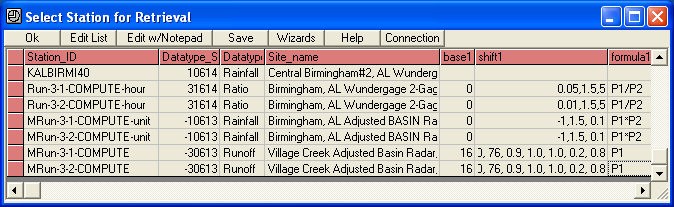
Multiple Model Runs with Multiple Traces
GetRealtime 3.0--If you would like to save multiple scenarios and variations on any of the
computations you can by simply attaching 'Run-1-1' or 'Run-1-2' to the
GetRealtime_setup.txt file's 'Station_ID' like 'RUN-1-1-COMPUTE-unit'.
If you would like to use these 'Run' data as input for further 'Run's then use 'MRUN-1-1-COMPUTE-unit'.
What the Run tells GetRealtime is that the results will be written to the
GetAccess database 'm' tables instead of the usual 'r' tables. 'M' being for
modeled data and 'R' for real data. The new 'm' tables have fields for a Run_ID
number and a Trace number. Having both a Run ID and a Trace ID may be overkill
but both are available if needed. If you use the same 'run_ID' and 'trace'
value all the values will be deleted and replaced when ran. So maybe having
multiple 'run_ID's isn't so far fetched after all.
In addition to your normal rtables output, if you would like to
save what is being computed or forecast then instead of 'RUN-1-1-COMPUTE-unit'
you could use just 'RUN-Compute-unit'. The mtables will also be
populated with the same data using the 'run_ID' = julian day and the 'trace_id'
incremented when run. This could be handy for keeping multiple NWS-Forecasts
during storm events to see how the forecasts panned out. GetGraphs can add
these Runs as traces for display. To save a run only a few times a
day in batch, then use something like "Run-1,7,13,19-FORECAST-NWS... This will
save to the Mtables 4 times a day at hours 1, 7, 13 and 19. The comma
separating the hours is important so you have to save at least two times a day. The forecast
will still be updated as usual in Rtables.
Now to use these 'Run' data as input for further
runs use 'MRun-1-1-'
instead of Run-1-1- to both read and write from the mtables. No change to
the 'rsite' table is needed. Mrun for Compute,
Snowmelt, and Route will use the mtables with these limitations:
Limitations on Mrun input:
Compute Runoff:
uses default
ET or rtable for ET
Route:
uses the same routing control file
Snowmelt:
only uses precip from mtable other parameters from rtable
startup swc, snow age, and albedo if any from rtable
To view your 'm' table values in GetAccess, use the check box 'M_Tables'
in the upper right of screen. Selecting your data uses the same steps
as 'r' data beginning with Run selection, then Trace. I am sure refinements to
all of this will be needed so check back often. In fact, you may have just
stepped into a Monte Carlo or an Index Sequential. The tables are rigged and
ready.
Try the Runoff Wizard's 'What If's' for your site to automate how all the
parameters affect runoff. Select 'Save to M_Tables' so you can send them to Excel
for comparisons as all traces or by dsid's. Don't be afraid to try it all you
like because I have automated Run_ID deletions.
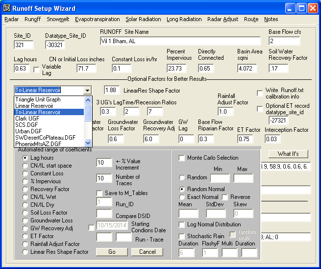
Update 1/12/2013 Stochastic Hydrology--In addition to the %
increment method, GetRealtime now has 3 Monte Carlo methods for varying any of
the runoff coefficients and the rainfall record for calibration or for
stochastic runoff:
1) Random--generates a random value between the
Max and Min. Any value is as
likely as the next.
2) Random Normal--generates a random NORMAL number 0-1 as a standard normal
deviate, computes the skewed deviate K, and uses the mean and std deviation for
V=Mean + StdDev * K.
3) Exact Normal--assures no outliers will be produced. It computes the plotting
position P as P=(rank-.4)/(N+.2) for each trace value 1 to N, computes the
standard normal deviate for P, computes the skewed deviate K, and uses the mean
and std deviation for V=Mean + StdDev * K. The 'Reverse' checkbox allows
reversing the ranking order so you can make a few traces at the top or bottom of
your Prob curve and then close GetRealtime with out running all 100,000 traces.
Log Normal uses the mean, std dev, and skew for log values, but you enter the
mean and std dev as unLogged values.
The 'Max' and 'Min' values are not limits to methods 2 and 3. GetRealtime limits
the values generated to zero or greater and less than where needed (Curve
Numbers).
For stochastic runoff you can vary the single rainfall record using any of
these Monte Carlo methods on the P1 'Rainfall Adjust Factor'. You can use
multiple runs how ever you dream up to use it. For soil starting conditions you
could make say 10 runs of 1 or 30 days with Run-1-1, Run-1-2... out to 10 with a
varied (monte?) runoff coefficient like initial CN. Now you have 10 traces with
starting conditions in table mday that you can select from by setting the
'Starting Conditions Date' and its Run ID and Trace ID. If Run ID is blank then
the starting conditions will be for the date in the usual rday table.
To create one or multiple rainfall temporal distributions you have to create you
own rainfall record just like your current rainfall record above and apply the
Monte Carlo. Where you get this record and normalize it and how many sounds like
work to me. Lots of ways I guess. If anyone can put all this to good use I
am certainly open to adding anything more that is needed.
For a trial storm you could try using GetAccess to load some runit radar
5-minute values for any DSID for 1 day, select Graph, Update database with
Excel, and you will have an updatable runit list of dates and values. At the top
of the Excel sheet you can change the 4-10xxx value to 4-10yyy where yyy is your
new DSID or change the dates and use the same DSID. Now we need some rainfall
record, so do an Excel 'File', 'Open' and load from your GetNexrad folder the
text file GetNexrad_6hour_Dist.txt and copy one of these 6-hour normalized
storms of 1" back to the Edit workbook and you can update these values back to the
GetAccess table runit. Now all you need is the mean, std dev, and skew for monte
carloing this normalized storm. You could take the noaa atlas 2yr 6-hr and 100yr
6hr and compute the mean and std deviation with zero skew but to add in the 10yr
and figure the skew is beyond me. You could try my free GetRegression's
Probability option on my More Stuff page and trial and error the stats for skew.
For Las Vegas I found by GetRegression trial and error:
N0AA Atlas 6-hr storm: 2-yr=0.79" 10-yr=1.30" 100-yr=2.12" ... that the log10
mean is the 2 year, std dev in log10=0.165, and the skew is 0.38 just to show
you can trial and error it. So for GetRealtime Monte Carlo the mean and std dev
are these UNlogged values 0.79, 1.462 and 0.38 skew with 'Log Normal
Distribution' CHECKED.
If you would like to familiarize yourself with these normal deviates (oxymoron)
and their devination you can download this
Monte Carlo Excel sheet and look at the simple VBA code for what is going
on.
What is really needed is a simple stochastic rainfall pattern generator to avoid all the
leg work with coming up with real rainfall distributions. I searched the online
stochastic literature, but with my limited math skills I could not find much of
anything useful. I did find a very clear
article by the NWS on their
Probabilistic Quantitative Precipitation Forecast that stated that rainfall
frequencies could almost always be fit with a special case of the Gamma
distribution. This made me recall that the Gamma distribution could also be used
to fit the triangular unit graph... that made me think of my new found Linear
Reservoir hydrograph that looks a lot like the power function of the Gamma
distribution. So putting 2 and 2 together with a random number between +-0.5
gives VIOLA!!! The ACME Linear Reservoir Stochastic Rainfall
Generator guaranteed to satisfy your every rainfall problem with just
one easy parameter:
Rain2=Rain1*e^(random*F ) where F is
a 5-minute shaping factor and series normalized to 1".
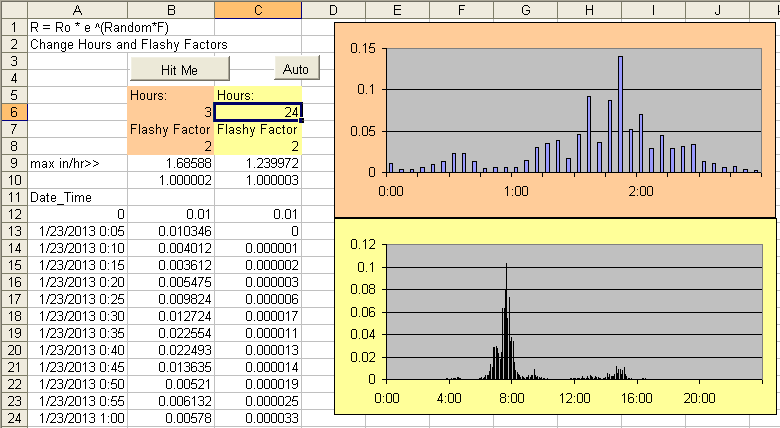
I was dumbfounded as to its actually working meaning it sure looks like rain.
One parameter between 0 to 3 should come close to any storm type of any duration
with a 5-minute time step. For California 24-72 hour stratiform storms try a
F=0.3. For frontal thunderstorms east of the Rockies of 6-12 hours try a F=1.0.
For desert Southwest sporadic monsoon thunderstorms of 3 hours try a F=2.0.
Now that we have a simple
but usable stochastic rainfall pattern generator any of the 'What Ifs' can be
combined with the 'Stochastic Rainfall' option. I would imagine though that one
of the Monte Carlo options with the 'Rainfall Adjust Factor' chosen is how it
would normally be used. The stochastic rainfall values will be saved to the
M-tables if you choose that option. And again, if you do not need the unit
values saved then uncheck the 'Write Unit Values' to speed things up.
A couple of uses come to mind, one is where you
hold the 100-year 6-hour rainfall P1 adjust constant and let the pattern do its
thing, and another where you know the 72-hr max annual rainfall totals mean,
stddev, and skew and let the Monte Carlo generate 72-hr totals for each run and
let the pattern again do its thing. Longer periods like 90 days may take some
more thinking, but you can give it a try. This is starting to get out of
hand but I guess I should add randomizing the number of storms in a 90-day period
but I am running out of room for checkboxes.
Update 10/31/2013--GetRealtime 3.2.1--If you would like an
*Alert* printed and beep sounded on values exceeding a given
value now you can. To do this you need to modify the 'GetRealtime_setup.txt'
file's field 'Datatype_name' like:
KALHUEY99;10612;Rainfall>0.5"-hour; Hueytown, AL
Then whenever the hourly value exceeds 0.5 the alert is printed to
'GetRealtime_Alert.txt'. If you want to check a running sum like for 24 hours
then use this:
KALHUEY99;10612;Rainfall>0.5inch-hour-24sum; Hueytown, AL
You can use this with any datatype and you can use tables hour, day,
daymax, and unit in
the Datatype_name. The values are checked as they are being written so it's only
for the period retrieved. You can maximize the GetRealtime window and use the
'View Alerts' button to view the 'GetRealtime_Alert.txt'. You can delete this
file as needed. If you are clever, you can automate reading this file and
doing something about it. Remember you can shell GetNexrad.exe and GetGraphs.exe
and they can write to the web.
To have the alert message sent from your email provider as email or cell
phone text add the following email address info to
GetRealtime_Setup.txt:
Alert Address= MailTo, MailFrom, ServerPassWord, SmtpServer, SmtpPort (25 or 465
for SSL) , optional info
Example: Alert Address= joe@yiho.com, me@lu.com, mypassword,
smtpout.myserver.net, 25, http://www.getmyrealtime.com
Here's a list of
SMTP
mail servers to find your email provider.
The MailTo value using SMS cell phone text message could be
for AT&T...
MailTo: 1234567890@txt.att.net
Here's a list of cell phone SMS
MailTo
addresses.
and add -email on the end of the 'Datatype_name' like:
Rainfall>0.5"-hour-email
For multiple MailTo's, separate each email address with a
single space.
To add a flag like Flood Level with different levels 1,2,3...
set your datatype_name cell like:
COMPUTE; -11340; Rainfall>1.1-unit-12sum-email; Hot Creek, CA
ROUTE; -1340; Flow>-daymax-email-50cfs Minor,80cfs Moderate,140cfs Major;
Hot Creek, CA
LOOKUP; -2331; Stage>-unit-email-0.85ft Minor,2.2ft Moderate,5ft Major; Hot
Creek, CA
LOOKUP; -2333; Stage>-unit-email-0.85Minor,2.2Moderate,5Major; Hot Creek, CA
You should stick to alert levels 'Action', 'Minor', 'Moderate', and 'Major' but
you can use what ever you wish. And becareful how you use the '-' field
separator.
All database tables will find the first occurance of each level. A special case
is using DAYMAX with a single value (not levels). In this case the Maximum for
the period being written will be returned as the alert value.
For email CC's and BCC's add these to the GetRealtime_setup.txt:
Alert Address CC= space separated list
Alert Address BCC= space separated list
And to ignore these CC's and BCC's use '-emailTO' instead of
'-email'.
And if you would only like to include CC and BCC for a level 2 or higher use
-emailTO2 or -emailTO3 etc.
When running in batch mode, the alert emails will be sent twice, then turned off
for 12 hours, then back on for twice again and so forth. You don't want to get
100 emails for the same darn thing do ya. Alerts begin checking values 1
hour ago or if Sum then the sum period plus 1 hour ago. If you would like
to start checking alerts earlier (or later) than 1 hour ago, then use the
GetReatlime_Setup.txt line where -2 is 2 hours earlier than NOW:
Alert Start Time=-2
Note:
GetRealtime is using the Microsoft CDO library (cdosys.dll) that ships on most
Windows PC's. If you get an error I would recheck that your MailTo and MailFrom
values look like email addresses and that you got the right port 25 (non SSL) or
465 (SSL) value as supplied by your email provider.
To display the Alerts on GetGraphs add 'Alert' to the GetGraphs
setup line like:
1 ;-2329 , 2609, Alert ;Stage;Big Cr at 24th St;......
BUT...Alerts cannot be displayed on the very first
Getgraphs setup page so choose the 2nd
or other graph page for alerts.
The alert value and and time issued will be plotted as triangles for dsid -2329.
If the alert value issued does not change then no triangle will be added until
the issued value changes or is a day old. The alerts are read from
...\GetRealtime\GetRealtime_Alert.txt.
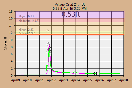
The GetGraphs chart above shows what happens with a 3-Hour Nowcast when a squall
line forms and you're not paying attention (needs Maddox 30R75 winds aloft
adjustment).
Update 11/16/2013--GetRealtime 3.2.2--has been updated to write
its MS-Access database values to a Hec-DSS data file (v6-32bit) in real-time. So you can use
my GetRealtime to achieve all your flood forecasting system needs, or you can
now use GetRealtime to just provide Hec-HMS or Hec-Ras your
GetRealtime radar rainfall or runoff and let them take it from there.
Here is an example GetRealtime_setup.txt to write the DSS data files (No
'rtable' change needed):
COMPUTE-Put-unit; 30619; Runoff; Village Creek Upper Sub Bham, AL; -1;
VillageCrSubs.dss
COMPUTE-Put-unit; 30618; Runoff; Village Creek Lower Sub Bham ,AL; 0;
VillageCrSubs.dss
The -1 means delete the DSS file first and the 0 means just add to it. You will
need to reinstall over yours the FULL GetRealtime 3.2.2 download to get the
needed heclib.dll support files. No need to uninstall, just reinstall.
If you want to write 15 minute flows to DSS instead of 5 then use 'Put-15unit' like
this:
COMPUTE-Put-15unit; 30619; Runoff; Village Creek Upper Sub Bham, AL; -1;
VillageCrSubs.dss; P1+10.24
Now we have a DSS file for Hec-Ras or Hec-Hms.
Update 11/23/2013--Running Hec-Ras Unsteady Flow projects from
GetRealtime. To run your Hec-Ras project from GetRealtime you will
first have to write a Hec-DSS file (v6-32bit) of your inflow hydrograph as discussed above.
Running Hec-Ras requires version 6.x and GetRealtime.exe > 4.4.2.
Download GetRealtimeRas41.exe to use Ras 4.1. Download GetRealtimeRas5.exe
to use Ras 5.x. Ras 6.1 installed on my Windows 10 but Ras 6.1 would
install but not start up with out error on my Windows 7. In Win 7 I
renamed sqlite3.dll in C:\Windows\SysWOW64 and Ras 6.1 installs and starts up
without error. I don't know what program sqlite3.dll belongs to.
When changing Ras version set Initial Conditions to an inflow value to update
restart files and Run the Geometry process and save all. Current
GetRealtime.exe references Ras version is 6.4.1.
HEC-RAS tip for beginners: For routing multiple subbasins create one long reach
with at a minimum one x-section at the top and another at the bottom. Subbasin
unsteady hydrograph inflow Boundary Conditions can be one at the top of the
reach and all others at chosen interpolated x-secs as
**Side Inflow** boundaries. Only took a week watching Youtubes
without ever finding a good example before figuring this out myself. DO NOT try
the obvious way of multiple side reaches with Joints (that way lies madness).
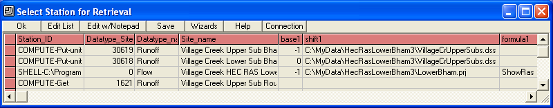
For this example our Hec-Ras project file will be created in this folder and
name:
C:\MyData\HecRasLowerBham3\LowerBham.prj
...have GetRealtime 'Put' a dss file of inflows like this:
GetRealtime_Setup.txt line:
COMPUTE-Put-unit; 30619; Runoff; Village Creek Upper
Sub, AL; 0;C:\MyData\HecRasLowerBham3\VillageCrSubs.dss
Now that we have a DSS
boundary inflow file in our project folder we can start Hec-Ras and create a
project and save it where we put the inflow DSS file. As a quick example for a
Hec-Ras unsteady flow project start up Ras:
1) File> New project and locate the
folder above and save project.
2) Edit> Geometric data> River Reach ... and draw a line and double click to end
and enter the River name and Reach name.
3) Cross Section> Options> Add a new Cross Section ... and give it station id
and add the xs data. Then hit Apply Data.
4) Repeat step 3 for a downstream xs by Edit> Options> Copy current cross
section> Add new Cross Section and Options> Adjust Elevations.
5) Exit and from the Geometric Data menu File> Save geometric data... and close
window.
6) Now we need a unsteady flow plan BUT... before that we need to set the run
TIME WINDOW or else you cannot select the plan boundary inflow hydrograph. To
set time window Run> Unsteady Flow Analysis> and on the Simulation Time Window
set the start and end times and be sure to click on the year label and set to
something reasonable. Once you set the time window date and times, close the
menu.
7) NOW!!! Edit> Unsteady flow data> click on the upstream Boundary Condition
cell, click Flow Hydrograph, Select DSS file and Path, click on the little Open
File ICON, and select the dss file VillageCrSubs.dss from our work above and you
should be able to Select highlighted DSS pathname(s), and plot them. If you can
plot them then they are in the correct time window we set in step 6. Click OK...
and then OK.
8) Back at the Unsteady Flow Data menu, click on the downstream xs Boundary
Condition cell, Normal Depth, and enter the channel slope. And save by File>
Save Unsteady Flow Data... and close window.
9)From main menu, Run> Unsteady Flow Analysis> enter Short ID, and click all 3
Process to Run, set all 3 Computation Settings to 5-minutes... and I think we
are set to go... now hit Compute!!! Hot Dam!!! it ran.
10) Whew... now to watch a water level movie, click View> Cross-Sections> and click the Animate
Button. Cool eh! I'm sure the experts are chuckling on the steps above but it is
how I got a Hec-Ras project to work so if you know better, just skip all the
craziness above and create a project.
Now to run Ras.exe from within GetRealtime.
GetRealtime_Setup.txt line:
SHELL-C:\Program Files\HEC\HEC-RAS\5.0.3\ras.exe; 0; Flow; Village Creek HEC RAS
Lower Sub; -1;C:\MyData\HecRasLowerBham3\LowerBham.prj
The -1 means watch it run, 0 is hide it. When GetRealtime is run it will open
the .prj file, find the current plan (p01), open the .p01 file and set the
Simulation Date time window to the current retrieval period, and away it goes.
The Ras.exe is not directly shelled but is referenced by it's HEC River Analysis
System... which is Ras.exe but makes all it's objects available to call. I used
the GetRealtime 'SHELL' command in case other programs can be shelled
using the same setups in the future.
But if you enter 'ShowRas' in the 'formula1' cell setup like:
SHELL-C:\Program Files\HEC\HEC-RAS\5.0.3\ras.exe; 0; Flow; Village Creek HEC RAS
Lower Sub; -1; C:\MyData\HecRasLowerBham3\LowerBham.prj; ShowRas
Then the Hec-Ras program WILL be shelled so you can admire your project after
GetRealtime ends.
You can also delete unwanted files before the Ras run like this formula1:
showras, delete.dss, delete.bco01
Delete.dss automatically also deletes the .dsc catalog file. I found that
deleting the DSS output file makes things simpler in the beginning.
If you want to shorten your Ras run time to just around the peak then add
'PeakN' to the formula1 list like:
showras, delete.dss, delete.bco01, Peak12
For this Peak12 example the Ras run will start 12 hours before the max peak of
all runoffs and flows and 3*12 or 36 hours after the max peak for the run. This
will speed things up if all you want are peaks for Ras Mapper.
Now to get the Ras DSS file results back into
GetAccess database add...
COMPUTE-Get; 1621; Flow; Village Creek Upper Sub
Routed, AL
The GetAccess table 'rsite' for this Get is:
621; 1621; Village Creek Routed Subs, AL; 1; flow; cfs; cubic feet per second;
GetUnitHecRasLowerBHAMrouted.txt; COMPUTE-GET; 6; NC; 0;
For the GetUnitHecRasLowerBHAMrouted.txt filename. This file in your GetRealtime
folder will read:
Hec-Ras Routed Bham Upper Sub to Gage
Put Table: runit
Get Database_connection:C:\MyData\HecRasLowerBham3\LowerBham.dss
Get SQL: /VILLAGE CR AIRPORTTOGAGE/10/FLOW/DAY1/5MIN/SHORT2/
END
The Get SQL is the DSS 'path' name that you can copy from HEC_DSSvue.exe. The
/DAY1/ part does not matter because it gets replaced with blank because it is
not needed. Note: Do Not Include 'HMS' In Your Title.
If your Ras project takes a while to run and you don't want to start at the
beginning of the runoff period, then you can create a HotStart file.
1) To use a HotStart (aka Restart File) with date and time
under the Ras Menu 'Run':
Run, Unsteady Flow Analysis, Optioons, Output Options, Restart File Options:
Check Both (or at least first) Write Intial Condion file...
Set Hours from beginning of simulation: [ 1 ]
Hours between writes: [ 1 ]
Now GetRealtime will set run start date time to match a .rst hotstart file
datetime<= to your startdate.
2) For the first time w/o a .rst file, set your Initial Conditions option to
'Enter Initial flow distribution'.
3) Run your project.
4) Reset your Unsteady Initial Conditions to 'Use a Restart File' and
select the rst file.
5) Save you project.
In GetRealtime_setup.txt add 'hotstart' to the delete list
in 'formula1' cell like: delete.dss, delete.bco01, hotstart
Now when ever you shell Ras, it will start on the new
.rst hotstart file datetime<= to your startdate. The old hotstart .rst files
older than 7 days will be deleted at the end of each time run if you add
'delete.rst' to the formula1 cell. To run starting with beginning of the runoff
period set by GetRealtime's runoff comps, just remove 'hotstart' from the
formula1 cell setup... but be sure your last hotstart written is at base flow or
who knows what will happen!?!?
Additional HotStart options to add to the deletes are:
,Peak n,
This will get the maximum runoff for the run period and start RAS n hours before
the peak and end RAS 3*n hours after the peak.
,Now n1-n2,
This starts RAS n1 hours before the current run time and and ends RAS n2 hours
after the current run time. Example: ,Now 1-3 This starts 1 hour earlier and
ends 3 hours later.
If you need a higher low flow to avoid instability problems,
then use a P1+50 where needed on the upstream dss PUT and then a P1-50 on all
the GET's.
And to skip running RAS when not needed, see the
Station_ID 'IF'. This allows skipping the next N lines of the
GetRealtime_setup.txt if peak flow does not warrant unsteady routings or stage
mappings.
If you would like to capture the image of your RAS Mapper window (Ras 5 only) at
the end of the Ras run then add the option ,RasMapperPic to
save for display by GetGraphs.
This will capture the image to png like this:
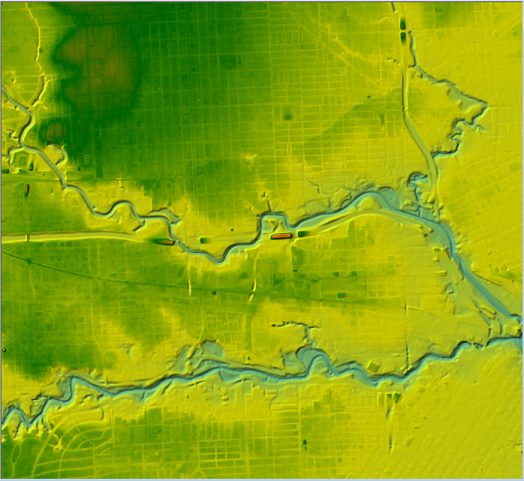
Update 1/8/2014--Running HEC-Hms runoff projects from GetRealtime.
To run your HEC-Hms project from GetRealtime with gage or adjusted radar
we first have to write a Hec-DSS file (v6-32bit) of your rainfall hyetographs as
discussed above. For this example our HEC-Hms project file will be created in
this folder and file name:
C:\MyData\VillageCr\VillageCr.hms
First have GetRealtime 'Put' a dss file
of rainfalls with base -1 overwrite like this
GetRealtime_Setup.txt line (-1 on first sub-basin only):
COMPUTE-Put-unit; 11616; PRECIP-INC; Village Creek;
-1; C:\MyData\VillageCr\MyVillageCrRainfall.dss
Now you can create your
VillageCr.hms project and get it running. Set the 'Time-Series Data', 'Precipitation
Gages', 'Gage 1', 'Time Window', 'End Date' to a future year so you won't have
to deal with it till then again.
Once your project is running using the DSS
rainfall you can now run GetRealtime to automate HEC-Hms, so close HEC-Hms.
Important Dec 5, 2018: HEC-HMS.cmd version 4.3 does not seem to run script (Failed
to register GDAL/OGR for use (truncated path?)). I contacted COE for help and their system ran
fine. Maybe next HMS update will fix my problem. 4.3 runs on my
Win10 but not my Win7. Tested Hec-HMS 4.5 shelling in Win7 and works fine.
I think HMS 4.3 was using way too much environment variable space for my Win7 to
handle.
Update Feb 16, 2022: HMS 4.9 was running fine on Win7 for a few weeks and
I did something and now it won't. Win10 never did shell 4.9. Back to
HMS 4.8 until the next version. Sometimes version 4.9 will shell ok after
rebooting. You might try uninstalling all older HEC-HMS versions?
For Windows 7 with HMS version 4.9 and greater copy HMS version 4.8 file
HEC-HMS.cmd to your new HMS install folder. Apparently the newer CMD file is for
Windows 10 only.
GetRealtime_Setup.txt
line:
SHELL-C:\Program Files\HEC\HEC-HMS\4.1\hec-hms.cmd; 0; Flow; Village Cr
HEC HMS Example; -1; C:\MyData\VillageCr\VillageCr.hms, Control_1.control, run
1, 5-Minute; delete.dss, delete.log
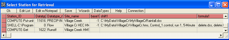
The first 0 is a DSID that is not used. The base1 -1
displays the HMS computation window and run log, a 0 turns it off. The shift1 is the
HMS project path name, control file, Run ID, and time-step. The formula1 are optional
deletes. The 'run_1.log' file is always deleted before running so you can
quickly see if things went wrong. You can use any valid run id. The time step is
always 5-minute for radar but you could use steps like 10-Minute, 15-minute,
1-Hour, 6-Hour.
Shelling
Hec-HMS in batch mode is not as
straight forward as you may think. HMS is not an ActiveX component as is HEC-Ras
and to shell I had to use the Windows API to get a process handle
for completion notice of the script HMS runs (GetRealtime_hms.script). The
script file is generated automatically if it does not exist. Warning! If
you copy your HMS project to another folder DELETE
GetRealtime_hms.script before running the GetRealtime shell or your
project path will not change.
After GetRealtime
completes the shelling of HMS then the results of the run will be in
VillageCr.dss. To retrieve the results back to GetAccess HDB, follow the steps
in the HEC-Ras example above.
Your rtable setup file will look like this:
Hec-HMS Village Cr
Put Table: runit
Get Database_connection: C:\MyData\VillageCr\VillageCr.dss
Get SQL: //SUB1/FLOW/07JAN2014/5MIN/RUN:RUN 1/
END
And again the
/date/ is just a place holder that gets replaced.
The letters 'HMS' have to be in the title line.
HMS will cut off your recession if you don't include enough starting days. To
automate the start day to avoid this, include at least one GetRealtime runoff
subbasin setup and you can adjust this sub's lag time and area to
provide sufficient recession time.
I think my GetRealtime continuous CN loss,
unit graphs, optimized Modpul,
snowmelt, stochastic rainfall, Monte Carlo methods, AND DATABASE are better than HMS so I hope you give them a try. Perhaps
you may prefer the HMS routings to mine so you could use HMS to do the routings
of GetRealtime generated runoffs. Lots of possibilities exist now that HEC-Ras
and HEC-Hms can be automated. Alert and HEC-ResSim users may see how automating everything
in real-time with a 7-day 5-minute forecast of runoff would be a pretty slick
deal. But the real key to success here is good adjusted radar rainfall so all this
work is useless if you can't get that done and done right and you're the
only man in a position to do it.
Update 2/3/2015--Running HEC-ResSim reservoir projects from GetRealtime.
To run your HEC-ResSim watersheds you will want to put the needed inflows to
your DSS file (v6-32bit), shell Ressim, and then get the results back into GetAccess from
the simulation DSS file. So just like HMS and RAS here is a GetReatime_Setup.txt
example:
*******; ********; *********; ***HEC-RESSIM********
COMPUTE-Put-hour; 30801; Flow; Browns Creek; 0;
C:\MyData\base\Testing_of_functions\rss\functiontest.dss
COMPUTE-Put-hour; 30801; Flow; Browns Creek; 0; C:\MyData\base\Testing_of_functions\rss\TestOfResSim\simulation.dss;
lookback=1
SHELL-C:\Program Files\HEC\HEC-ResSim\3.1\HEC-ResSim.exe; 0; Flow; Browns Cr;
-1; C:\MyData\base\Testing_of_functions\rss\TestOfResSim.simperiod; lookback=1
COMPUTE-Get; 1912; Flow; Browns Cr HEC Ressim Example
*******; ********;
*********; ***********
The GET file could read as:
Hec-Ressim DS CP2 flow
Put
Table: rhour
Get Database_connection:
C:\MyData\base\Testing_of_functions\rss\TestOfResSim\simulation.dss
Get SQL:
//DS END OF MAIN STEM/FLOW/01FEB2015/1HOUR/FUNC_TEST-0/
END
As of yet, I cannot automate the HEC-ResSim.exe executable, only shell it, and
let the user select his project and run it. When the project is closed,
GetRealtime will then get the results. The first PUT above to
'functiontest.dss' is probably optional after you get your project built and
running. I hope to figure out a ResSim Jpython batch file. If you know Jpython
and can create your *.PY file then the GetRealtime shell could be like:
SHELL-C:\Program Files\HEC\HEC-ResSim\3.1\HEC-ResSim.exe
"C:\MyData\base\BatchRunControl.py" "C:\MyData\base\Testing_of_functions"
Here is a COE Jpython example with documentation, only it is INTERACTIVE and not
what I need but somewhere to start:
BatchRunControl.zip
I think Hec-RTS is the Army's attempt at doing what GetRealtime is way better at. ;-) ...after
reading this...
HEC-Rts Draft
Just use GetRealtime... or shell Ras and Hms if you must. I don't
think calibrating your losses on the come, worrying about dead gages, using 4 hour old USGS flows,
and knowing your radar grid is an hour or 2 outdated after it starts raining and
the dam is about to break is such a good idea. If the radar loop bearing down on you
and NWS QPF says run for the hills, I would take them at their word. You can
always blame the NWS later like state governors do. But if you're running
Grand Coulee I guess you can afford such luxuries. Actually the soil
adjustment to match the USGS current base flow idea works pretty neat and has
been added to GetRealtime.
If you don't believe me then you could use GetRealtime as an overall check on
conditions, a middle ground 2nd opinion, or as complete redundant backup system.
With your data in a real database your in-house users can
actually make use of it.
Automate EPA-SWMM: Once you build your SWMM model and get it
running (or see the Nashville SWMM example) you can then edit your
GetRealtime_setup.txt to PUT, SHELL, and GET like:
COMPUTE-Put-unit; 11801; intensity; Lumped Nasville Basin; -1;
C:\GetNashville\NashvilleSWMM\TS1.dat
SHELL-SWMM; 0; Flow; Nashville Subs; -1; C:\GetNashville\NashvilleSWMM\MyTutorial.INP
COMPUTE-Get-SWMM; 1801; Runof; Nashville SWMM subcatch #1; 0;
C:\GetNashville\NashvilleSWMM\MyTutorial.out; Type=Catchment,
Item=0, Variable=4
COMPUTE-Get-SWMM; 1806; Flow; Nashville SWMM Outflow; 0;
C:\GetNashville\NashvilleSWMM\MyTutorial.out; Type=Node,
Item=4, Variable=4
Copy your C:\Program Files\EPA SWMM 5.1\swmm5.dll
and vcomp100.dll
to your PC's
system32 or your syswow if 64-bit or if you prefer to your path.
SWMM PUT setup:
To create a SWMM data source file for rain, the datatype_site_id is 11801 as
GetAccess data source. The datatype_name is either intensity or
cumulative. I have never heard of a volume of rainfall (gallons?) so the put
file will have unaltered GetAccess incremental rainfall if volume, so go with intensity to be safe. Be sure
your SWMM project's rain gage property Time Interval is set to
0:05 for 5-minute radar or 0:10 for Canada 10-minute radar. The base1 -1 means overwrite the SWMM data file (actually
overwrite is the only option), the shift1 is the SWMM dat file
name and the file name itself (TS1) is used as the SWMM Station ID.
SWMM SHELL setup:
SHELL-SWMM will run SWMM from 'swmm5.dll' which you should copy from C:\Program
Files\EPA SWMM 5.1\swmm5.dll and vcomp100.dll to your PC's system32 or your syswow if 64-bit or
if you prefer to your path. The rest of the fields are not used except shift1
which is the SWMM input file name (*.INP). GetRealtime will edit the *.INP
file's Start and End times to the period being run.
SWMM GET coefficients:
The datatype_site_id is 1801 for the GetAcces database, the base1 is ignored,
shift1 is the SWMM output file (*.OUT), and formula1 are the SWMM coefficents
for the get.
You should probably check the unit values in GetAccess with the SWMM GUI object
report table values to be sure you got the right TYPE, ITEM, and VARIABLE ID
numbers. I'm a rookie here but it seems if you click on a map object, then
report, table, by object, will display the VARIABLES in order with 0 ID is the
first VARIABLE and the TYPE seems to be shown in Oject Category. Apparently you
have to inspect the INP file for ITEM count. You may also notice that the
GET-SWMM does not need a Get File and the parameter_code in GetAccess
table rsite is ignored.
TYPE = type of object whose value is being sought:
subcatchment, node, link, system
ITEM = argument identifies items of a given TYPE that are
reported on by consecutive numbers starting from 0, which are assigned in the
same order as the item appeared in the SWMM 5 input file. As an example, suppose
that a system contains 5 junction nodes with ID names J1, J2, J3, J4, and J5
that are listed in this same order in the project's input file, but output
results are only requested for junctions J2 and J4. Then an itemIndex of 0 would
retrieve results for J2 while an itemIndex of 1 would do the same for J4. Any
other values for itemIndex would be invalid. For System items the itemIndex
argument is ignored.
VARIABLE = depends on the TYPE being sought and are listed in
the Output File as follows:
· Number of subcatchment variables (currently 6 + number of pollutants).
· Code number of each subcatchment variable:
0 for rainfall (in/hr or mm/hr),
1 for snow depth (in or mm),
2 for evaporation + infiltration losses (in/hr or mm/hr),
3 for runoff rate (flow units),
4 for groundwater outflow rate (flow units),
5 for groundwater water table elevation (ft or m),
6 for runoff concentration of first pollutant,
...
5 + N for runoff concentration of N-th pollutant.
· Number of node variables (currently 6 + number of pollutants)
· Code number of each node variable:
0 for depth of water above invert (ft or m),
1 for hydraulic head (ft or m),
2 for volume of stored + ponded water (ft3 or m3),
3 for lateral inflow (flow units),
4 for total inflow (lateral + upstream) (flow units),
5 for flow lost to flooding (flow units),
6 for concentration of first pollutant,
...
5 + N for concentration of N-th pollutant.
· Number of link variables (currently 5 + number of pollutants)
· Code number of each link variable:
0 for flow rate (flow units),
1 for flow depth (ft or m),
2 for flow velocity (ft/s or m/s),
3 for Froude number,
4 for capacity (fraction of conduit filled),
5 for concentration of first pollutant,
...
4 + N for concentration of N-th pollutant.
· Number of system-wide variables (currently 14)
· Code number of each system-wide variable:
0 for air temperature (deg. F or deg. C),
1 for rainfall (in/hr or mm/hr),
2 for snow depth (in or mm),
3 for evaporation + infiltration loss rate (in/hr or mm/hr),
4 for runoff flow (flow units),
5 for dry weather inflow (flow units),
6 for groundwater inflow (flow units),
7 for RDII inflow (flow units),
8 for user supplied direct inflow (flow units),
9 for total lateral inflow (sum of variables 4 to 8) (flow units),
10 for flow lost to flooding (flow units),
11 for flow leaving through outfalls (flow units),
12 for volume of stored water (ft3 or m3),
13 for evaporation rate (in/day or mm/day)
The Army and I think alike when it comes to thumbnails on the radar screen
(GetNexrad):
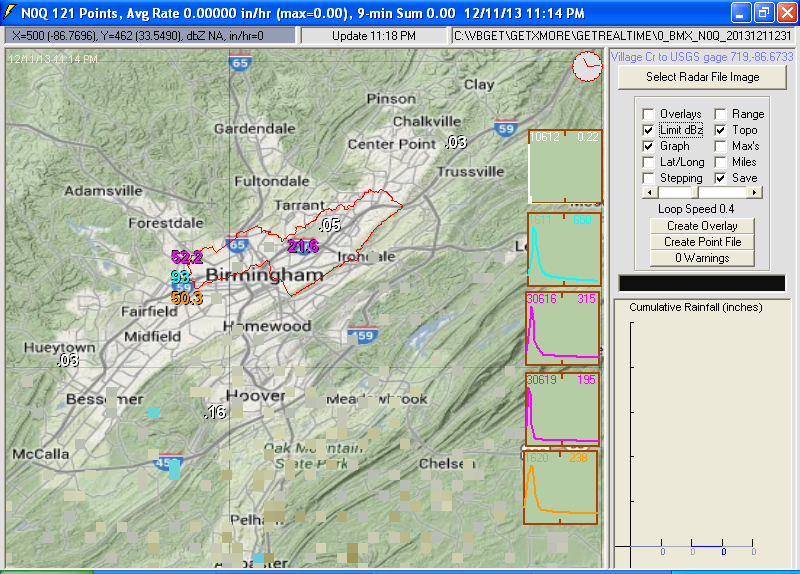
Or just a quick look at all your subs and adjusting rain gages on the radar:
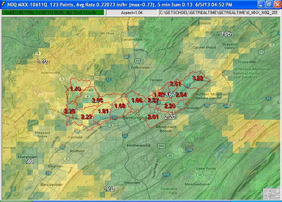
And the pages of rainfall, frequencies, and runoff graphs and web info in
GetGraphs:
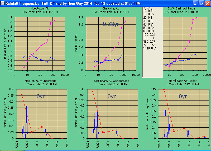
Other Shell Examples:
The first time you run these Shells you will need to run GetRealtime.exe as
System Administrater and give permissions when prompted. Update Jan 27,
2021: These shells (not Hec or Swmm) will time out after 3 minutes. You can
change the 3 in GetRealtime_setup.txt (save it first if missing).
For Windows 10 you may need to change security settings Allow App Through
Firewall.
The GetRealtime_setup.txt lines can use the GetNexrad and GetGraphs command
lines. Only the first field (Station_id) and the last field (base1) has
any meaning so don't over think this:
SHELL-C:\GetRealtime\GetNexrad\GetNexrad.exe -2; 0; Pic;
Nashville Radar Window;-1
(Saves to file and you could then add the png file to your GetGraphs setup list.)
The -2 means capture the window, a -1 would
mean capture just the radar image. To FTP to your
GetNexrad ftp setup include your password: GetNexrad.exe -2 mypassword; ...load default and save window to png file and FTP it:
SHELL-C:\GetRealtime\GetNexrad\GetNexrad.exe -2 MyPassword; 0;
Some Pic; Nashville
sub 1;-1
The ending base1 -1 displays GetNexrad,
0 hides it but only when saving the
radar image, not the whole window which will always display.
Update 1/5/2021 now GetNexrad can use multiple setup files so you can do radar
selections and surface obs and save to GetNexradFilesxxxxxx.txt and then reload
GetNexrad from a command line with the new setup flilename. A simple example
would be to include a radar image of the whole USA radar, NWS flood sites, and
QPF rings and it updates automatically.
New command lines could be:
GetNexrade.exe -2 GetNexradFiles33.txt mypassword (ftp)
or
GetNexrade.exe -2 GetNexradFiles33.txt (no ftp, just create
png for GetGraphs)
old way:
GetNexrade.exe -2 mypassword (use old default
GetNexradFiles.txt and ftp)
Likewise, GetGraphs can be shelled similarly and png's FTP'd:
SHELL-C:\GetRealtime\GetGraphs\GetGraphs.exe 1 MyPassword; 0;
graphs; Nashville GetGraphs
(where 1 is the pause in seconds between GetGraphs paging.
there are no window or image or display hide options.)
On GetGraphs you have to select 'Auto Paging' and check the 'Write page image on
update' and then fill out and 'Save Web Info'. This creates the file
'GetGraphs_autoweb.txt'. Then you're all set up and your web password if needed
is supplied by the GetRealtime SHELL command.
And if you don't want to FTP a particular page use FTP_OFF on
the GetGraphs_setup.txt page line.
To shell and wait for BAT or SCRIPT files:
SHELL-CopyMyFIles.bat; 0;Copy
my Pic; Pic of Tallapoosa basin; 0
(SHELL dos commands like COPY can be put in a BAT file.)
SHELL FTP EXAMPLE: To Shell FTP and wait for it using
GetRealtime.exe, put the following in a script text file like
C:\mydata\MyFTPer.txt :
---------
open ftp.getmyrealtime.com
user myrealtime mypassword
cd MiscImgs
binary
put C:\myImgData\Graphimage.png
bye
-------
The GetRealtime_setup.txt line would be:
SHELL-ftp -n -s:C:\mydata\MyFTPer.txt; 0; MyInfo; Send me to somewhere; 0
Note there is no space between s: and C:. Like wise NEVER use spaces in file
names or you are just asking for trouble in life.
To automate retrievals from the GetAccess database from a batch
file or directly from GetRealtime.exe you can use my 3 programs
GetFromAccess.exe/GetFromAccessNOW.exe and
GetFromAccessSQL.exe. Like the names imply, the first needs your dates to
retrieve or days relative to now, while the other uses any SQL statement. GetFromAccess.exe can even
create HEC-DSS files. The advantage of the SQL method is the use of SQL
functions like NOW(), SUM(), and MAX(). Like give me the past 6 hours... give me
the sum of the past 6 hours, give me the max of the future 48 hours. These are
intended for automating retrievals for FTP'ing to your WebSite. Run
the Exe's with no command line to display help examples.
For help with GetFromAccessSQL batch look at these files in the zip download:
Help_GetFromAccessSQL.txt
SQL_Now_Examples.txt
MySQLGetAccessTXT_EXAMPLE.bat reads as:
GetFromAccessSQL -11361 -30361; SELECT * FROM rhour WHERE datatype_site_id=DSID
AND date_time BETWEEN (Now()-0.25) AND Now() ORDER BY date_time;
MyTextOutTest.txt
To create an Excel file try .xls instead of .txt:
GetFromAccess rhour, -11321 -11323 -11326, 2016-11-01 00:00, 2016-11-02 00:00,
myTest.xls
As an example of putting a data file on the web you could use this setup line in
GetRealtime:
SHELL-C:\GetGraphs2\GetFromAccessNOW.exe rdaymax, 10347 -10347 17340 -23363
11363 1332 -1360, -2, 5, BurroCrNOW.txt, mypassword; 0; To Web; Put text file on
web; 0
Note that I had the exe in my GetGraphs folder where my GetGraphs_autoweb.txt
file has the needed web info.
To create a small BABY.mdb database file and FTP it you can use
PutFromAccessNOW. It will read your
large database and create a small version of values only for that run. This
could be handy to FTP a small MDB file to someone else running GetGraphs with
just the needed current values for graphing.
NWS Forecasts:
Update May 15, 2024 - The NWS 7day hourly forecast has
returned to service. Also try SpotWX as Forecast-GFS but you may need to buy him a cup of coffee.
The NWS 7-day forecast dsid's
and table rsite parameter_codes:
9,
10 or 11 qpf
16 dewpoint
17 temperature
18 humidity
19 wind direction
28 windspeed
26 cloud-amount
NWS snow model data is above for 48 hour Melt and
SWE, Depth and Density, Rainfall and Snowfall, Air Temp and Surface Temp
NWS forecast of stage and flow add the NWS gage ID
like this:
FORECAST-NWS,wsbt2; 1409; Forecast Flow; USGS Flows below
Reservoirs
If your datatype_id from table rsite is
1 then flows are retrieved, else stage.
I would expect one already has the USGS flow in table rsite as only the forecast
values are saved.
NWS flood flow forecast info: https://water.noaa.gov/map
Update May 13, 2026: You will need the
curl downloading tool if you don't have it in your GetRealtime folder.
GetRealtime can add the NWS
hourly QPF's directly
and here is the setup. The -2 is a time shift. I chose adjusted radar for the QPF
so there is no time shift on that so I had to add it here. You could also put the
QPF in the basin radar DSID and the gage adjustments will not change it.
For flow and stage the date_times are adjusted to your PC's
time zone from Zulu for you.
Very important update 7/24/2017: The NWS QPF forecast
FORECAST-NWS must come before the radar Nexrad-ESX with Nowcasts (and HRR-ESX)
in the setup because of the addition of the HRRR 18-hour forecast. See MRMS-HRR
below for proper setup sequence.
FORECAST-NWS; 11616; Rainfall; Birmingham 3G Adj BASIN
Forecast; -2; 33.52, -86.82, 3
(Always put temp, humidity, wind, cloud-amount AFTER rainfall
forecast so distribution will be read.)
Note the Lat,Long. I would use the same Lat,Long for a general area for each
subbasin. The NWS QPF forecast grid width is about 4 miles and updated
hourly at hh:45. GetRealtime checks to see if the Lat,Long has changed before
re-retrieving the QPF. Place all your QPF's for the same Lat/Long together so
the QPF's only get retrieved once. And like GetNexrad which
distributes each 6-hour QPF, GetRealtime also distributes as 0=average,
1=Denver 2-hr design storm, 2=Dallas 4-hour, 3=Vegas 5-hour, 4=California
6-hour storm, and 5=etc. You may need to copy the file
GetNexrad_6hour_Dist.txt to your GetRealtime folder. In the
example above, 3 means Vegas distribution. You may note that the hourly QPF is
the same value for 6 hours, hence 6-hour QPF. GetRealtime detects each new
6-hour starting time and restarts the distribution. The nearest 6-hours may be a
little screwy as the distribution assumes it will go for 6 hours when in fact it
may reset after 1 hour as a new 6-hour QPF begins.
I can see I have a lot to learn about forecasting. The problem is the NWS QPF is
for 6 hours. The distributions above work great for periods more than 6 hours
out, neglecting peak timing. For the next 1 to possibly 6 hours those
distributions can zero out the forecast just as it should be peaking. So the the
first 1 to possibly 6 hours of a forecast will be distributed by heavily
weighting the first hour as below and reduced each hour with the distribution
not used. For Vegas the
first hour of the next 6 would be 3X, then the 2nd hour 2X, then 1X, then zero.
Distribution 5 and higher will use average for up to the next 6 hours.
Storm_Type FirstHour NextHourReduction
1-Denver 5 4
2-Dallas 4 2
3-Vegas 3 1
4-California 2 0.4
5-E & Beyond 1 0
This means when starting the forecast you could be doubling your forecast for
periods less than the full 6 hours so during events you may want to switch to
Average storm type and/or edit the first 6 hours with the Forecast Wizard to
account for history which is very easily done. I'm trying to help.
Once the end of the current 6 hourly forecast changes, then the distributions kick
back in. So the next 6-hours is critical and you should learn more than I know
about this! As luck would have it, you can use Run-FORECAST-NWS
(instead of FORECAST-NWS) to save each forecast in the M-Tables from which you
can learn something.
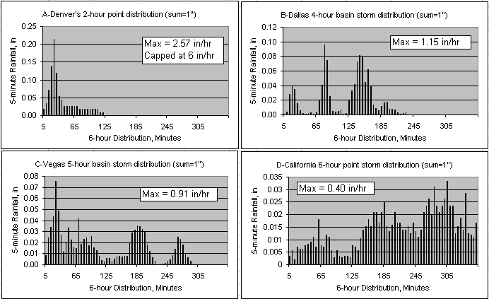
The above 2-hour distribution was taken from Denver, CO's
Drainage Manual (noaa atlas) and adjusted to 1 inch. The others are
actual storms. Also, the 5-minute values are capped at 6 in/hr and a beep
will sound if check 'Beep On'.
What I've found so far: The NWS forecasts are for 6 hour
periods beginning 0:00, 6:00, 12:00, and 18:00 hours locally. Sometimes they
break them up to 3 hour periods at storm start or end. You definitely want to
use a storm distribution beyond the first 6 hours. And you probably want to use
it for at least the first 1 or 2 hours with history. Make note of the peak
runoff and keep that peak in mind as you go through the next 6 hours. Don't get
faked out and think you are way over shooting because these NWS forecasts are
damn good! Look at the regional radar mosaic 2-hour loop and point rainfalls up
wind with GetNexrad. But in the end the original 6 hour forecast with storm
distribution will probably give the closest peak runoff so err on the high side
until the closing of the 0, 6, 12, and 18 times above. Use the Forecast Wizard
forecast edit to keep the original 6-hour depth until you know the radar is
changing to the high side or reduce the last 3 or 4 hours if needed to keep
things in line with the radar mosaic. You could use the 0-Average storm
distribution and manually edit it so you know where you are at each hour but
don't use it as a real forecast. If you use an 0-Average distribution, then look
at my front loading methods above and adjust for history. When you screw up,
just get the forecast again and start over. History will show how much of the
forecast is left to expect based on the 0,6,12,18 periods. And use a
Run-Forecast on the first sub and Run-Compute or Run-Route to save all your
messes for posterity.
http://www.hpc.ncep.noaa.gov/html/fam2.shtml#qpf
Form the Forecast Wizard Setup you can edit the next 6 hours of
forecast manually. Here is a list of ways to change forecasts:
0) 1, 2, 3 hour automated Nowcasts using winds aloft (GetRealtime).
1) Storm distribution of NWS.
2) Time shift.
3) 5-minute Forecast value adjust as P1*x.
4) 1+ hour storm track forecast (GetNexrad).
5) 6 hour QPF of any amount starting any time (GetNexrad).
6) A wundergage up wind with a time shift???
7) Edit next 6 hours with Forecast Wizard.
8) Use the Forecast Wizard Edit 6 hours to copy the first forecast 6 hours to
all other forecasts.
9) Forecast Overwrite checkbox on Scheduled Batch menu overwrites all edits with
NWS Forecast.
And remember to use Run-FORECAST-NWS to save forecasts to the
'M' tables for post event analysis of where you went wrong and use
GetGraph's menu 'Add Trace' to compare. To
view the previous RUN on GetGraphs startup automatically, add ',RUN' to your
GetGraphs_setup.txt line for that DSID:
4 ;-11301 ,-10301 , Run ;Rainfall; Sub1 Adj & UnAdj & Last Forecast; 0 ; .....
Note that when running 2 or 3 separate GetRealtime.exe's in batch mode
that you stagger their start times by 3 or 4 minutes to insure they don't
collide updating the GetAccess HDB database.
You can run Runoff, Routings, HEC-Hms, and HEC-Ras for the QPF's additional future days.
Besides precip, FORECAST-NWS can also be used for SNOWMELT comps based on the
datatype_id for temp, humidity, wind speed (and some other things). Always
list the precip QPF first if using a re-distribution from above or it has to
retrieve the QPF twice.
MRMS Multi Radar Multi Sensor products from NCEP:
A2M and
HRRR.
Both A2M and HRRR products are processed by Iowa Mesonet into ConUS images and
archived. Downloaded images use Iowa's map cutting web service for smaller areas
of interest (ConUS, 10-Regional, each Radr Site).
A2M is a 1-km 2-minute rainfall rate with 255
values. The setup Station_ID is
NEXRAD-ESX (for ESX radar). The table rsite parameter_code is A2M-Ridge2 with
MRMS-ESX station_id. Rain rates will be converted and saved as 5-minute rainfall
increments on a 1-km grid for the subbasin boundary (same as Nexrad-NCQ
boundaries). Level3RGB2RainRateA2m.txt is the rainfall rate color conversion
table.
HRRR is a
1-km 15-minute 18-hour FORECAST of reflectivity with 255 values (same
colors as N0Q) but archived by Iowa as a 2-km grid. The setup site_name is
HRR-ESX (for ESX radar). Rain rate reflectivity will be downloaded and saved as
5-minute rainfall for
the subbasin boundary (same as Nexrad-NCQ boundaries). HRRR forecasts can
also be downloaded using the SpotWx data source as values instead of images and
is much faster.
Both A2M and HRRR are processed just like
my Nexrad-NCQ images using the same
subbasin and gage boundary and point files. So if you have created NCQ
boundaries then nothing more is needed. So use product code NCQ Ridge2 with
LatLongPixels.exe and LatLongPixelsFromFile.exe when creating boundaries. See
GetNexradHelp for NCQ
boundaries. Both radars are adusted to your PC's time zone unlike the NWS
forecast.
You do not need to use A2M in order to use HRRR forecasts. In fact, A2M is
probably only wanted for locations over 100 (70 winter) miles from the radar, or
in mountainous terrain, or if you have no rain gages. HRRR forecasts can be
compared with my Nowcasts and NWS 6- hour forecasts. I'm just shortcutting on
this help write up as I am implementing both in code.
GetRealtime_setup.txt example lines:
A2M-ESX; -10361; Radar Rain; Burro Cr Sub 1 Rainfall QPE
HRR-ESX; -11361; Forecast Rain; Burro Cr Sub 1 Forecast Reflectiviy; 0; 6
Where ending 6 can be 1 to 18 hours of the available HRRR forecast period.
Table 'Rsite' A2M line:
361 -10361 Burro Creek Sub 1, AZ 10 rainfall in inches A2M-Ridge2 MRMS-ESX 3 AZ
Table 'Rsite' HRRR line uses SAME LINE AS ADUSTED RADAR DSID:
361 -11361 Burro Creek Sub 1 ESX Radar, AZ 11 rainfall in inches 31347,-10361 COMPUTE 3 AZ
I haven't priortized the HRRR forecast source code 24 to overwrite or not
overwrite Nowcast 14 or FORECAST-NWS 18 source codes so you will have to put the
HRR in the correct setup order of HRRR AFTER FORECAST-NWS. Source 14 overwrites
takes place during G/R ratio adjustment to raw radar for adjusted radar rainfall
and is last.
To clear all the Nowcasts and HRRR forecasts, use the 'Overwrite Forecasts' on
the 'Scheduled Batch' menu and run the FORECAST-NWS. Now you can rerun to
add the Nowcasts and HRRR forecasts and use the Wizards Forecast editor if
needed.
So I would order my 3 forecast sources like:
FORECAST-NWS; -11361; Forecast Rain; Burro Cr Sub 1; 0; 34.81,-113.17,5
A2M-ESX; -10361; Radar Rain; Burro Cr Sub 1 QPE;0; Nowcast 3, adjust type 3
HRR-ESX; -11361; Forecast Rain; Burro Cr Sub 1 Forecast Reflectiviy; 0; 6
Averages and Ratios...
COMPUTE; -11361; Rainfall; Burro Cr Sub 1 Adjusted ESX Radar, AZ; 0; -1, 1.0,
0.3, 0.0; P1*P2
GOOD ORDER:
FORECAST-NWS; -11101; Forcast Rain; Sub 1;
0; 34.8044,-85.0242,3
FORECAST-NWS; -11102; Forcast Rain; Sub 2; 0; 34.8044,-85.0242,3
NEXRAD-HTX; -10101; Radar Rain; Sub 1; 0; Nowcast 3, adjust type 3
NEXRAD-HTX; -10102; Radar Rain; Sub 2; 0; Nowcast 3, adjust type 3
HRR-HTX; -11101; Forcast Rain; Sub 1; 0; 12
HRR-HTX; -11102; Forcast Rain; Sub 2; 0; 12
COMPUTE;
-11101; Rainfall; Sub 1 Adjusted Radar, GA; 0; -1, 1.0,
0.3, 0.0; P1*P2
COMPUTE;
-11102; Rainfall; Sub 2 Adjusted Radar, GA; 0; -1, 1.0,
0.3, 0.0; P1*P2
LOOKUP (Update 2/11/2015): The LOOKUP command will read a
period of record from the HDB database and interpolate values from a rating
table. A tab delimited rating table for FLOW and Gage-Height might look like
this:
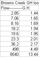
To convert a period of unit flows from the HDB a GetRealtime.exe setup line
could look like this:
Lookup-unit-log-log; 2805; G.H.; Nashville Routed Subs
The
HDB rtable line could look like this:

LOOKUP-Unit-Log-Log will convert the rating values to logs
before interpolating the log value of the lookup.
LOOKUP-Unit-Linear-Log is lookup linear flows but with log G.H.
LOOKUP-Unit-Log-Linear is lookup log flows but with linear G.H.
LOOKUP-Unit is linear flows and linear G.H.
You can use my USGSrating2lookup.exe
program to convert USGS Gh Shift Q ratings to lookup Q - GH files saved from
here:
http://waterdata.usgs.gov/nwisweb/data/ratings/exsa/USGS.09424447.exsa.rdb
Update 07/06/2015: Station_ID= IF
You can use the Station_id 'IF' in GetRealtime_setup.txt
select PARAMeters (routing filename) or to SKIP (or NOskip) the next N
stations on your setup like this:
IF; -1331; Flow Check; Sub 11 Flow Check For RAS Runs;
rdaymax; SKIP-34; P1<1000
For this setup the next 34 stations on the setup list will be skipped if the
maximum value in table rdaymax for the run period is less than 1000. The formula
'P1<1000' can be anything that evaluates to True or False. If table
'rdaymax' is used then SQL retrieval for 'P1' is automatically: SELECT MAX(value) AS
maxv FROM... This would be handy to skip a HEC-Ras unsteady flow and
mapping if the flow was not high enough to warrant it.
If table rdaymax is not used, then instead of the max for the
full run period, only the first value for the period is used from that rtable.
This could be helpful for running different runoff setups like unit graph type
or interception for very dry base flow conditions:
IF; -1300; Flow Check; Routed Base Flow for dry setups; rhour;
SKIP-4; P1<80
But in this case you will need another 'IF' in case the first 'IF' is false:
IF; -1300; Flow Check; Routed Base Flow; rhour; SKIP-4;
P1<80
COMPUTE-unit; -30301; Runoff; Oneida Cr Sub1, NY...
COMPUTE-unit; -30302; Runoff; Oneida Cr Sub2, NY...
************; ************; ************; *****Base Flow<80******
IF; -1300; Flow Check; Routed Base Flow; rhour; SKIP-2;
P1>=80
COMPUTE-unit; -30301; Runoff; Oneida Cr Sub1, NY...
COMPUTE-unit; -30302; Runoff; Oneida Cr Sub2, NY...
To reverse the SKIP-2 if true to never skip if true use
NOSKIP-2. Sometimes it much easier to write a true logic than a
false logic. For instance ALWAYS skip unless day is Monday, hour is 7, and
minute is less than 5:
IF; 0; Date Check; Check Date Time is True; rday; NOSKIP-1;
(Weekday(D)=2) and (Hour(D)=7) and (Minute(D)<5)
For very dry basin conditions try raising the SCS
initial abstraction form 0.2 to 0.4 with your 'IF'. Raising
interception will reduce groundwater so that might not be a good choice and IA
will increase groundwater.
To select a routing filename from the rtable Parameter_Code
string (f1.txt,f2.txt,f3.txt) then use the PARAM code like this for filenames
other than defualt 1:
IF; 0; Date Check; Check Month For Route Filename; rday; PARAM-2; month(D)=3
IF; 0; Date Check; Check Month For Route Filename; rday; PARAM-3; month(D)=4
IF; 0; Date Check; Check Month For Route Filename; rday; PARAM-4; month(D)>9
ROUTE-unit; -1110; Total Relase; BBQ Dam Modpul Total Outflow
Note no dsid needed if only checking date D.
D is the current date and time.
To check if an Alert message was issued use 'alert' as the dsid:
IF; Alert; Flow Check; Was Alert Sent; 0; NOSKIP-5; 0
Update 11/07/2015: Station_ID= SET-INTERVAL
You can use the Station_id 'SET' in GetRealtime_setup.txt to
set and reset the Batch minutes between retrievals like this:
SET-INTERVAL; -11611; Rainfall; Village Cr Big Sub Adj &
Forecast; -60,runit; 15; P1>.001
For this setup the Batch minutes between retrievals will be set to 15 minutes if
the maximum unit rainfall in rtable runit for dsid -11611 over the past 60
minutes is greater than 0.001 inches, otherwise it will be reset to the original
Batch interval.
This is handy to only do run retrievals once an hour then if there is rain for
the current run then set the next run to be in 15 minutes instead of 60. You
will want to place the SET line below the current retrieval for that dsid so the
current data will be available for checking.
The example here uses -60 look back, but you could do a +60 look ahead in table
runit, or +1 in rhour. It only checks the maximum value in the rtable for the
period from Now.
If you would like to go to even a more frequent batch run as the rainfall
increases, then add another batch time and function test to the SET line like
this:
SET-INTERVAL; -11611; Rainfall; Village Cr Big Sub Adj & Forecast; -60,runit; 15; P1>.001;
0; 5; P1>.2
The date of the next run will be writen to table rupdate field
'value' for sdid = -1. If you do a shell below the SET-Interval like
SHELL-GetFromAccessNow the next run date will be available.
Rain Gage Wind Speed Adjustment (update 6/10/2014):
Dr. David C. Curtis, DC Consulting, Folsom, California, referencing available
scientific literature concluded that a reasonable under catch estimate for
unshielded ALERT tipping bucket rain gauges is one-percent per mile-per-hour of
wind speed occurring at the height of the rain collector orifice for wind speeds
of 30 mph or less. For higher wind velocities, the effects are more uncertain.
More info on rain gage siting and adjustments:
http://tulliemet-perthshire.org.uk/main/images/InconsistentRainGageRecords.pdf
GetRealtime can adjust the 5-minute rainfall record by the formula P1*(1+P2/100)
where P1 is the 5-minute rainfall and P2 is the 5-minute wind speed. For a
Wundergage, it can be adjusted on download with the GetRealtime_setup.txt like:
It has been pointed out to me that P1/(1-P2/100) should be used:
With P1*(1+P2/100)
Precip = 0.85 * (1 + 15/100) = 0.98
With P1/(1-P2/100)
Precip = 0.85 / (1-15/100) = 1.00
KALBIRMI45;-9619; Rainfall Adj; Nucor Steel Wundergage; 0; 0; P1/(1-P2/100)
and the GetAccess table rsite for dsid -9619 as:
datatype_id= 10
parameter_code = dailyrainin,WindSpeedMPH
The rainfall need not be stored before adjustment but could also be done that
way with 'Compute-unit'.
Additional menu options available when window maximized:
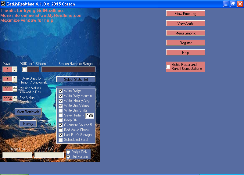
Additional menu items when 'Scheduled Batch' is checked:
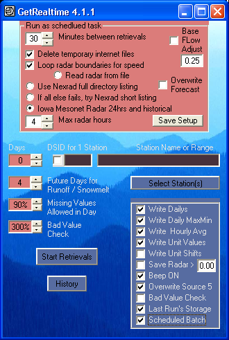
Uncheck 'Scheduled Batch' after setting options to run normally.
Metric Units (maximize window and set checkbox and save setup):
1--Radar rain saved as millimeters.
2--NWS-Forecast rain millimeters, Temp C, Dewpoint C, Wind KMH
3--Runoff input rain and ETo (if supplied) as mm's; saved as m^3/s.
4--Modpul routing rating table as
m, m^3/S and m^3.
5--Snowmelt inputs C, KMH, watts/m^2, mm; output mm's.
6--Radiation and ET inputs C, KMH; output watts/m^2, mm.
What I found needs changed from English to Metric:
1--Wunderground metric set with Temp C on Internet Explorer (not Chrome) on
website.
2--Gage/Radar ratio hail cap raised from 0.5" to 12.7mm.
3--Runoff coefficients NO CHANGES!!! base flow, area, and losses must be in cfs,
sqmi, inches.
4--Modified Puls rating columns are M, CMS, M^3 (ft*0.3048, cfs*0.028317,
af*1233.48)
5--Convert GetGraph's rainfall frequency tables, GetGraphs_Frequency.txt, to
millimeters and use log Y-axis scaling.
I have not done much testing of the metric units so be careful and let me know
if you spot a problem... better yet, learn to speak English, comrade!
GetRealtime.exe Configurations and Setups:
Update 1/25/2014--If you have made it this far, then it is time to get organized. Here is a
15 subbasin setup example using Excel that
puts some order to all this. Another tip of the hat to David in Alabama.
GetRealtime and GetGraphs setup files can now be pasted form Excel in Tab
delimited text format
Optional ways to run GetRealtime and the setup file for mixing retrievals:
1) To SKIP a station include an '*' with the first cell Station Code setup.
2) Move your unused stations below the END. (ex: snow seasonally)
3) Put all the runoff at the bottom and use a select on the upper.
4) What I do, create a separate installation for:
a) Wunder gages, run daily for 1 day.
b) Runoff, run for as long and when needed.
c) Radar, auto continuously every 1/2 hour (I am comparing old N1P)
or more often as needed.
5) With one installation, run auto continuous radar with selection, and then
daily or as wanted, start up GetRealtime.exe again select just the daily's.
(GetAccess wont let you update the same table like runit at the same time so you
have to look at the auto radar last run time by hovering your mouse over it.)
The files are WHERE?!?!?
GetRealtime.exe needs the point file (and boundary) in it's folder. I set up my
GetNexrad.exe to use the GetRealtime folder that does all my radar retrievals
for saving it's radar images. That way GetNexrad and GetRealtime have the same
boundary and point files.
If you don't want to go the trouble of building an Excel workbook to construct
your GetRealtime_setup.txt file and table Rsite, then build your
GetRealtime_setup.txt file first. Then you can select each line and add most of
the needed info to table Rsite. Also some Wizards will add all the needed info
to table Rsite based on the setup line.
I set up a separate GetRealtime.exe and folder for Wundergages and computations.
Update: Not sure why?
I don't do anything with C:\Program Files\. No files are registered anywhere but
the System.
You can install them over and over in C:\Program Files\ and then copy what is
new to all your working folders. If you want to stay in C:\Program Files\ then
just have GetNexrad save in the GetRealtime folder where all the boundary and
point files will be.
Maybe you can think of a better way for this like:
C:\GetRealtime\GetRealtime (w/boundary, point files)
C:\GetRealtime\GetNexrad (save images in GetRealtime)
C:\GetRealtime\GetGraphs (with GetFromAccessNOW.exe FTP automation)
C:\GetRealtime\GetAccess (the MDB file can be anywhere if shared but
usually here)
To have GetNexrad use the GetRealtime folder, select any image
from the GetRealtime folder even if it is a legend GIF for now. Then 'Save
Setup' and GetNexrad will then be using in common the GetRealtime folder.
And radar need not be retrieved when there is no rainfall.
Runoff computations will fill in zero rainfall for missing periods of rainfall
in the 5-minute record.
If you have made it this far, then it is time to get organized. Here is a
15 sub setup using Excel that
puts some order to all this. Another tip of the hat to David in Alabama.
That is all....
And again, it's important that the MS Access HDB
database be routinely 'Compacted and Repaired' to speed up downloads. The size of the
MS Access database doesn't seem to matter as much as how often data is being
updated. I retrieve about 100 stations every 1/2 hour with 5 minute unit values
(Nexrad). I find the down load time will double in about 2 to 3 days so I
'Compact and Repair' using the GetAccess.exe 'Connection' button every day or
two... so be smart like me. Look at your 'GetRealtime_errlog.txt' file to see
how your download times vary over time. Also see 'Defragment or Compact
First?' topic near the top in the GetAccess section. GetAccess 2.1.3 will now
check for fragmentation of the MDB database file and display it on the window
caption and can defragment it if wanted. After further review
I think all this must be an MS Access urban legend. I have not seen any change
in download times, but it is still a good idea to do it anyway and be smart like
me so you will have a backup of your database. And get a $10 USB memory
stick!
My MS Access database is 200 MB's with about one years worth of data.
Wikipedia says MS Access 2003 can handle 2 GB's or 10 more years. We shall see.
MS Access 2010 still uses our 2003 file format. One option to
reduce the database size is save the database file every year and then delete
all the unit values and keep going so historical unit values would be available
if ever really wanted in separate files. (as if Windows will never die,
remember DOS)
And my term 'HDB' stands for something I acquired from a bygone era, Hydrologic
Data Base. I should use the MS Access file name MDB... which stands for...
MYHydrologic Data Base... or something.
Good luck … and with any luck…
Rainy days are here again!!!
END
Some additional page links about
ET and Nexrad Radar help and comparisons:
List of How To Videos on Youtube
Help Page for GetNexrad.exe
Nexrad Rainfall to Tipping Bucket Comparison
ET and Radar Rainfall along the Lower Colorado
River, AZ-CA
Nexrad vs Tipping Bucket and Rainfall-Runoff Comparison
Blue Ridge Mtns, NC
Nexrad Rainfall-Runoff Comparison Las Vegas
Valley, NV
Nexrad
Rainfall-Runoff Comparison San Jouqin Valley, CA
Nexrad
Rainfall-Runoff Comparisons in northwestern Arizona
Nexrad Snowfall Comparisons in western
central Sierras, CA and Fargo, ND
WEBSITE MAP


WU USGS USBR NWS GoC USCS
CWRD COE
More Free Downloads
Comments/Questions
Email: carson@getmyrealtime.com
Label