|
|
A Step by Step Real-Time Radar Rainfall Setup Example... All the required Windows
softwares are available free on my web Downloads. (need to get
started with adjusted radar rainfall?
Start here.)
For this setup I will let you read the wise words of this quy and then I will
show you a radar rainfall setup for the basin he discusses. The steps will be
concise as possible here but you can refer to the GetRealtime Help web page for
more info on each step.
http://uwtrshd.com/assets/stormwater-runoff-modeling-accuracy-for-udfcd.pdf
And note his Table 3 Rainfall Totals for you distributed model afficianados
where 1-km radar error varied at 7 USGS rain gages for this small basin from
+188% to -13% for this one thunderstorm so never believe radar has a simple bias.
This is specially true for these fast developing thunderstorms at Denver. I
have noticed for other radar studies the area averaged radar is much closer to
the average of the rain gages than at any one rain gage. This also illustrates that
the blind use of off-the-shelf radar is something you better not do either so
you better learn how to adjust it yourself. It's as simple as 1,2,3...
err... 16.
Steps for setting up the Harvard Gultch lumped radar rainfall basin:
1) The basin was planimetered using my free GetMapArea
(Load/Save Map, Paste From Clipboard the web image below) using
the schematic below and these street intersection's Lat/Long's located
on the screen diagonal taken from
Google Earth for setting the x and y image scale in one step:
Dartmouth and University= 39.660339 , -104.959463
Evans and Holly= 39.678465 , -104.922252
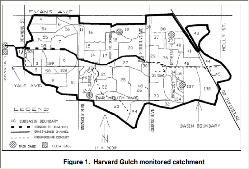
The longest stream course was also digitized from high elevation to outlet and
upstream and downstream elevations taken from Google Earth as shown here on
GetMapArea's 'Runoff Hydrograph' form.
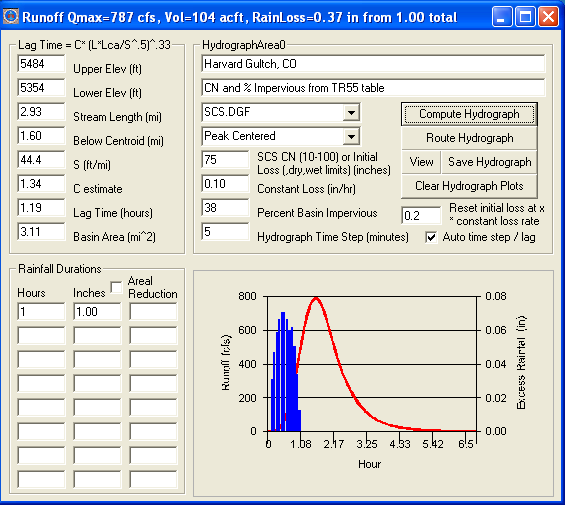
2) Runoff parameters: Using GetMapAreas's unit graph methods, the Lag Time is computed for us as
1.19 hours, the SCS dimensionless graph was selected beacause
we won't be calibrating the hydrograph's fast responce shape, the SCS Curve
Number loss method is estimated as 78 as a starting soil storage just above dry conditions,
0.10 constant loss, and 38% impervious for urban and the computed hydrograph is
shown. You may have a much better lag time method (not time of concentration) and you should use it if you
do because half the stream length is streets, storm pipes, and lined channels so my 1.19 hour lag is way too long. A better C estimate of 26*Manning's n = 26*0.025 for
the street/pipes and cobble natural channel combination
(0.015+0.035)/2 would give a
lag time of 0.58 hours and so we will use 0.58 hrs.
I looked up the soil survey as Silt Loams where mapped from
this great online source:
http://websoilsurvey.nrcs.usda.gov/app/
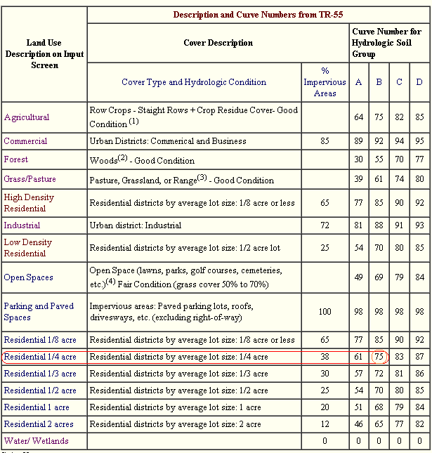
and CN and % impervious from an
SCS - TR55 table (the TR-55 urban manual has a
good CN overview):
https://engineering.purdue.edu/mapserve/LTHIA7/documentation/scs.htm
Silt loam (Soil B) has a flow recession Carson Recovery Factor of 0.17 from my
web Help page table for a constant loss rate 0.1 in/hr:
Example of using the soil survey and the table above for estimating the soil
recovery factor if we had more than one soil type:
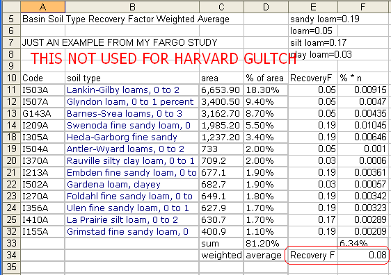
Look up Soil B silt loam 1/4 acre residential on a SCS Curver Number
table:
I forgot to check my other studies and used my default 0.1 in/hr
ConstLoss and 0.2 RF before thinking instead of 0.17 RF from Carson's
table above and remember recovery rate is the
ConstLoss*RecovFactor product. This means if you set your Constant Loss at
0.5 then your RecoveryFactor would be 0.04, not 0.2. From the TR-55 Curve Numbers for soil B silt
loam above for 1/4 acre
residential we have a % impervious of 38% and CN=75 as our Dry Condition
( I know they say it is a mid condition veg wise and dry conditions should have
a lower CN but the lawns and parks are watered and probably even closer to CNwet
conditions so stay tuned).
**** Fraction of % Impervious Directly Connected for
urban areas has been added posthumously ****
I added 'The Directly Connected Impervious Fraction' to
GetRealtime that the author discussed about cascading planes. This allows the
fraction of the %Impervious not dicrectly connected to be removed from the
excess and added to infiltration but limited by the pervious Curve Number loss method.
A big tip of the hat to Ben Urbonas the lead in article's
author.
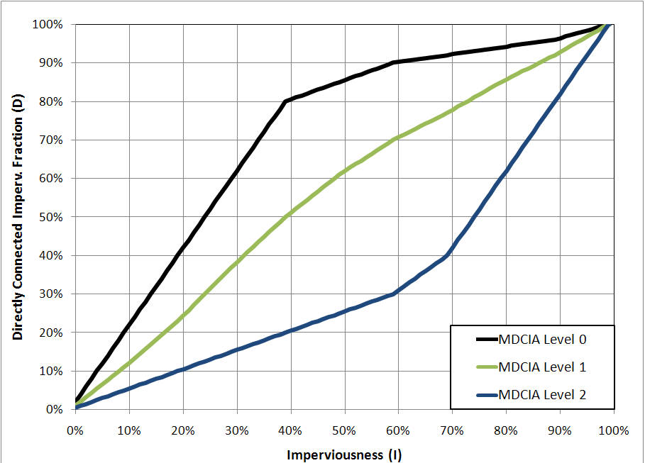
From Colorado Urban Drainage and Flood Control District for urban
catchment studies. The Levels in the graph are for the amount of Low Impact
Development added between the impervious areas and collecting channels. For 38% impervious shows
80% directly connected for minimal low impact developments (Level 0). This
was a very important addition and badly needed for urban areas.
Adjusting for Composite CN with unconnected impervious area (TR-55):
CNc= CNp+(Pimp/100)*(98-CNp)*(1-0.5R)
where
CNc = composite runoff curve number
CNp = pervious runoff curve number
Pimp = percent imperviousness
R = ratio of unconnected impervious area to total impervious area.
CNc=75+(38/100)*(98-75)*(1-0.5*0.2) CNc= 82.9
This addition regretfully has not been made YET (same as CF=1)
Note that just adjusting the CN values had little affect with 38% impervious and
that is the short comming of the TR-55 adjustments alone. You need to
reduce the % impervious and route it over the pervious using the CN loss method
which I could not come close to emulating without adding it to the GetRealtime
code.
Eventually this Cookbook will be revised and these off the shelf parameter
results better displayed. For now I think I got very lucky with the
adjusted Wundergage rainfall some how.
********************
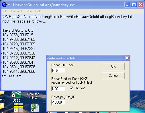
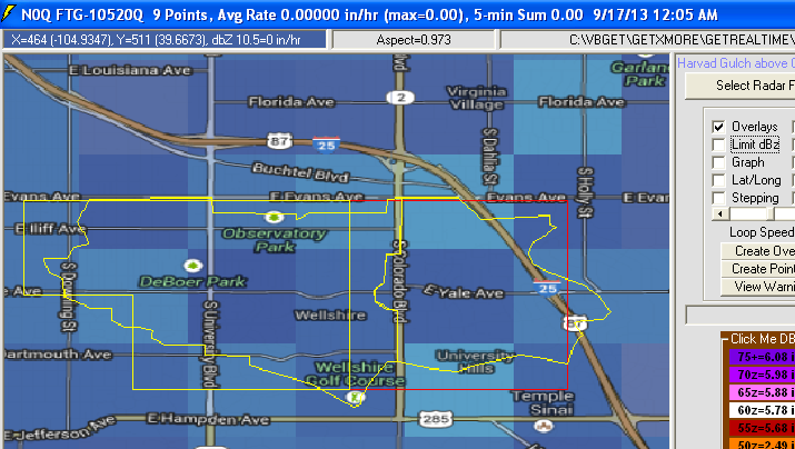
3) Now for the radar rainfall record. The planimetered basin
boundary lat/long text file from GetMapArea was converted by my free
LatLongPixelsFromFile to the Nexrad FTG radar's N0Q image pixel boundary
coordinates.
I try to stick to negative DSID's for computed values and positve for gaged.
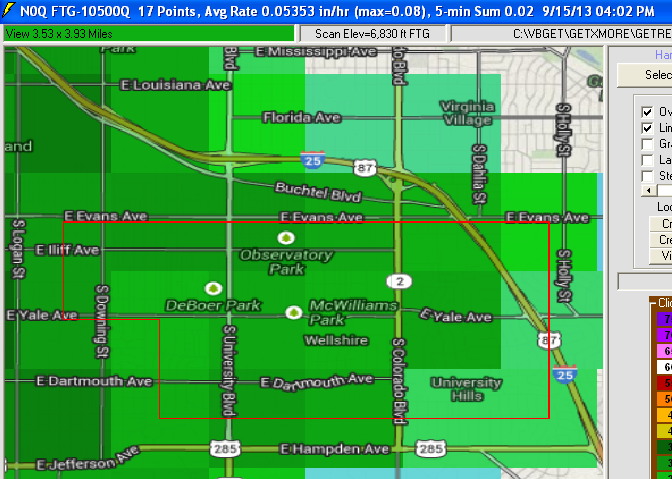
4) The boundary pixel file is then converted by my free
GetNexrad to radar image pixel point locations that is needed by my free
GetRealtime for computing the basin's 5-minute unadjusted radar rainfall record.
The Bounday file and the Point file should be in the GetRealtime radar image
directory. The 17 N0Q pixels each 1-km square (0.6 mile x 0.7 mile) that will be averaged for the basin
rainfall each 5-minutes is shown below:
Here's a better view of all rain gages and actual basin boundary in addition to
the required radar pixel boundary. You can add these features using my
free GetNexrad radar viewer:
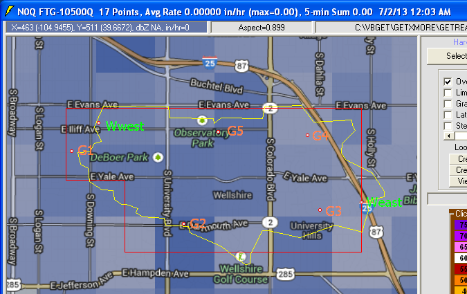
W=Wunderground gage, G=USGS gage.
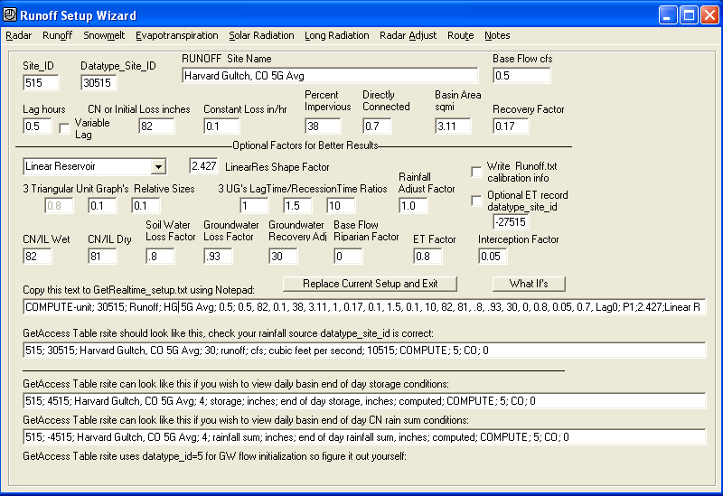
5) Now the setup for automating the basin radar rainfall record.
The GetRealtime_Setup.txt line is shown below.
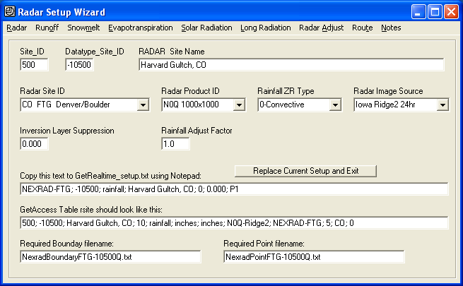
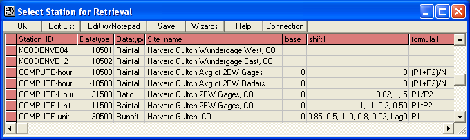
6) The GetAccess database table 'rsite' is edited as shown above (you
can't have one with out the other). You can copy and
paste the GetAccess Table rsite should look like this with GetAccess's edit menu
'Paste Clipboard'.
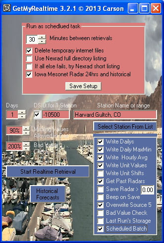
7) We are now setup to start retrieving real-time radar rainfall
or for an historical period. Run GetRealtime and select our Harvard Gultch and
retrieve the past 4 hours of basin's average 5-minute radar rainfall as below
(uncheck Scheduled Batch to watch the fun).
8) We now have a 4-hour record of 5-minute basin average rainfall that
is absolutely good for nothing because it needs to be adjusted. To do that we
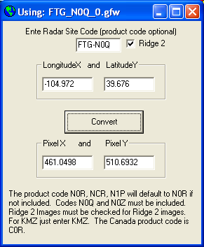
need gauged rainfall from at least 2 nearby Wundergages. Open this link to our
first Wundergage:
http://www.wunderground.com/weatherstation/WXDailyHistory.asp?ID=KCODENVE84
Over on the web page right find its Lat/Long location as 39.676, -104.972.
9) We need to set its pixel location on the FTG radar N0Q image
so start up my free LatLongPixels and enter the radar and lat/long values:
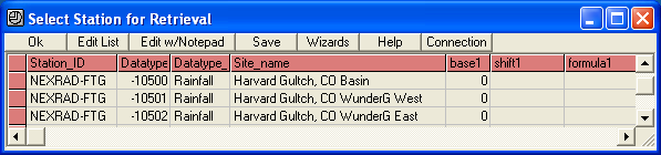
10) Copy the boundary and point files to the GetRealtime image directory
and add the info to the GetRealtime_Setup.txt and GetAccess table 'rsite'.
GetRealtime_Setup.txt:
NEXRAD-FTG; -10501; rainfall; Harvard Gultch Wundergage West, CO; 0; 0.000; P1
GetAccess table 'rsite':
501; -10501; Harvard Gultch Wundergage West, CO; 10; rainfall; inches; inches;
N0Q-Ridge2; NEXRAD-FTG; 5; CO; 0
11) Now we have the radar at the Wundergage. To get the actual
Wundergage record add these to the GetRealtime setup and GetAccess
table rsite:
GetRealtime_Setup.txt:
KCODENVE84; 10501; rainfall; Harvard Gultch Wundergage West, CO
GetAccess table 'rsite':
501; 10501; Harvard Gultch Wundergage West, CO; 10; rainfall; inches; inches;
dailyrainin; KCODENVE84; 5; CO; -1
Note that the Wundergage record is adjusted to my Pacific Time from Mountain
Time by adding the -1 in the rsite table cell 'time_shift'. The radar does not
need a time_shift because that is automatically adjusted to your computers time.
12) Repeat for Wundergage #2 KCODENVE12 as DSID -10502 radar
and 10502 gage.
NEXRAD-FTG; -10502; rainfall; Harvard Gultch Wundergage East, CO; 0; 0.000; P1
KCODENVE12; 10502; rainfall; Harvard Gultch Wundergage East, CO
and
502; -10502; Harvard Gultch Wundergage East, CO; 10; rainfall; inches; inches;
N0Q-Ridge2; NEXRAD-FTG; 5; CO; 0
502; 10502; Harvard Gultch Wundergage East, CO; 10; rainfall; inches; inches;
dailyrainin; KCODENVE12; 5; CO; -1
13) We now have records for the 2 Wundergages and their radar 5-minute
records. To adjust the basin average radar record we need to compute
the hourly average of the 2 Wundergage records and the hourly average of the 2
radar records at the gages. The setups are:
GetRealtime_Setup.txt:
COMPUTE-hour; 10503; Rainfall; Harvard Gultch Avg of 2EW Gages; 0; 0; (P1+P2)/N
COMPUTE-hour; -10503; Rainfall; Harvard Gultch Avg of 2EW Radars; 0; 0;
(P1+P2)/N
GetAccess table 'rsite':
503; 10503; Harvard Gultch Avg of 2 gages Wunderg; 10; rainfall; inches; inches;
10501, 10502; COMPUTE; 5; CO; 0
503; -10503; Harvard Gultch Avg of 2 gages Radar; 10; rainfall; inches; inches;
-10501, -10502; COMPUTE; 5; CO; 0
Note that the gage time is not shifted because it already was.
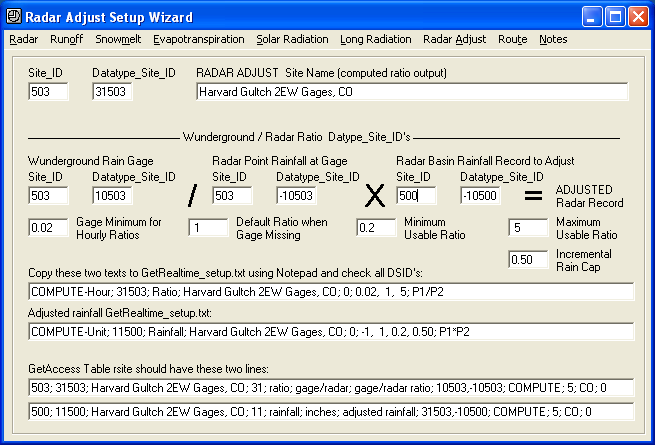
14) Now compute the ratio of the Wundergage and Radar hourly averages
AND adjust the average 5-minute basin radar with these setups.
I use datatype=11 for adjusted radar rainfall to help keep track of all the
different rain records.
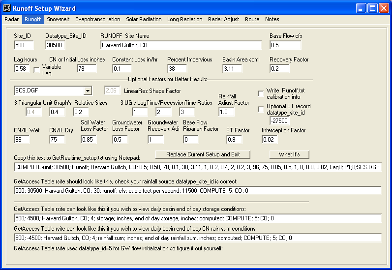
15) We now have adjusted basin average radar rainfall so all that is
left is runoff setup. Lag, CN_dry, Constant Loss, % Impervious, Area,
and Recovery Factor were found in Step 2 above. The other parameters are
general starting points from my expert experience, ha, along with a 0.5 cfs base
flow.
16) To review, here is GetRealtime_Setup.txt and GetAccess rsite
table:
I install a separate GetRealtime
(copy getrealtime.exe to another folder) for retrieving real-time radar.
This is so just the radar can be run in real-time each 1/2 hour but is no longer
necessary with Iowa Mesonet:
GetAccess table rsite:
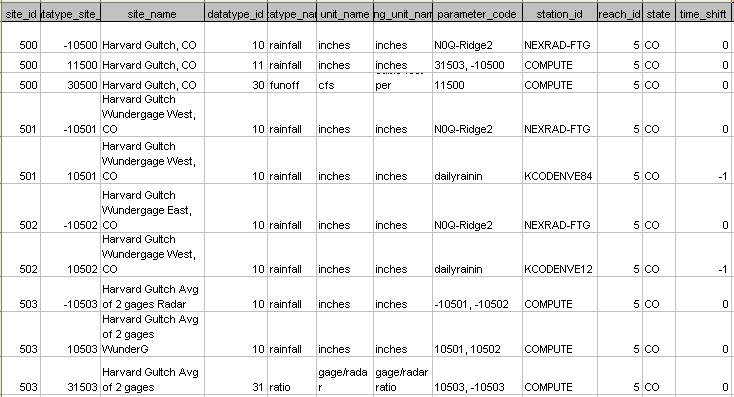
For your sanity's sake, it's a good idea to save the GetAccess table 'rsite' by
using the 'Graph/Table' button to TMP.out file, and then open it in Excel.
From here you can adjust column size and print out the table to a hard copy.
Now you can pencil in lines connecting the COMPUTE datatype_site_id's (DSID)
back to their owner's site_name and tack it up on your wall. You can go
crazy keeping track of more rain gages and computations if you try to keep it
all in your head. I do not have a printer so you see how I got this way.
You can also use MS-Access to open your database and copy and paste the table 'rsite' selected lines
into Excel directly like I did above (another big tip of the hat to David in
Alabama).
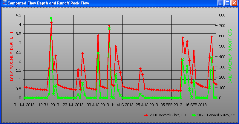
17) And now for the big finale... compute the basin runoff and
with your current radar rainfall and if no rain your runoff will look like
this. (radar need only be retrieved when it rains and at least 2 hours prior to
rainfall start if adjusting):
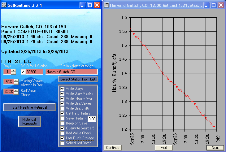
Congradulations!!!... you have just
graduated from the GetReal School of Runoff.
***********************************
SO HOW DID WE DO with our
off-the-shelf cookbook parameters??? (does not include % Impervious Directly
Connected factor or is 1. This explains the much too high peaks below 200
cfs.):
GetRealtime was run Jul 1, 2013 to Sep 25, 2013. The
full day's N0Q radar was retrieved from Iowa Mesonet for the days when there was
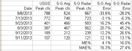
0.04 inches or more of rainfall for the two Wundergage average record. Here are the daily peak
flow comparisons with the USGS gage for the period:
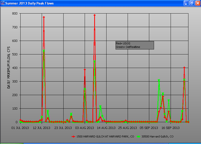
The large peak times
(lag) are all within 5-minutes so it looks like you under estimated the SCS Curve Number CN_dry;
live and learn. The TR-55 CN table for 1/4 acre residential = 75 did not
accout for the commercial area I quess but should be countered by the parks. The % impervious could be too high
or the 0.02 interception factor could be raised some for the peaks below 100
cfs (no pervious excess). Update: As usual, it turns out
our adjusted radar basin rainfall was 2 inches low for the 88 day period
compared to the 5 USGS rain gages so free is not always better, ha. Go talk to
the Wundergage owners. It's always the rain gages.
So say we had non-recording rain gages at the automated Wundergage sites that we
read at the end of each month for verification we could then adjust the
automated record each month. To make this cheating even simpler I will
compare the monthly sum of the the 2 Wundergage average record to the monthly
sum of the average of the 2 nearest USGS gages. I can then simply
use the monthly ratio value when I compute the 2 Wundergage average:
Example New July
GetRealtime_Setup.txt:
COMPUTE-hour; 10503; Rainfall; Harvard Gultch Avg of 2EW Gages; 0; 0;
1.42*(P1+P2)/N
|
Monthly Rainfall (Inches) |
|
|
|
|
|
|
|
WunderG |
WunderG |
WunderG |
USGS |
USGS |
USGS |
USGS/W |
|
2013 |
West |
East |
Avg |
at Gage |
Bradley |
Avg |
ratio |
|
July |
1.23 |
1.55 |
1.39 |
2.03 |
1.92 |
1.975 |
1.42 |
|
Aug |
0.92 |
1.79 |
1.355 |
1.87 |
2.16 |
2.015 |
1.49 |
|
Sep * |
3.07 |
4.05 |
3.56 |
3.8 |
4.76 |
4.28 |
1.20 |
|
note: WunderG East missing Sep 16, used WunderG West hourly values. |
|
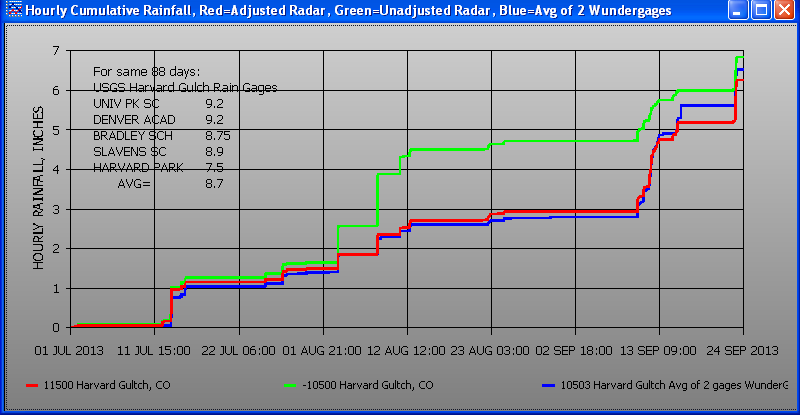
Based on the monthly ratios the adjusted basin radar rainfall was raised from
6.3" to 8.2" for the 3 month period:
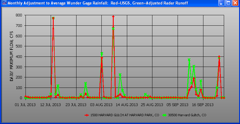
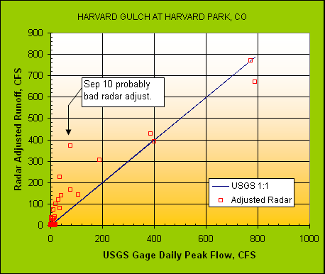
Not bad I think. Sep 10 radar rainfall
is probably too high although the hourly
ratio of 1.63 was well in line.
Note that all the peaks below 200 cfs have been subsequently corrected not by
radar adjustment but by cascading planes.
To evaluate our recession factor of 0.2
for soil recovery, a log plot look at the daily low flow
recessions is shown:
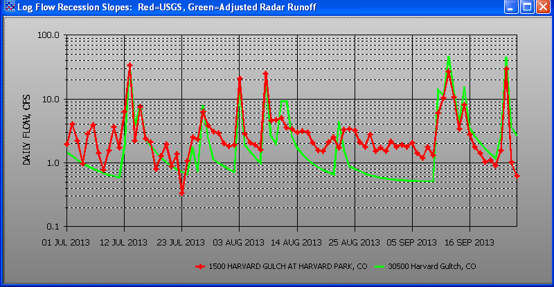
Not alot to go by on the recession slopes but the lower lows in July and the 3
or 4 days starting Sep 16 look like the RecessionFactor is in the pall park.
I'm guessing the base flow here is lawn watering that hides the full recession.
Because all of our large peaks compare relatively the same, antecedant soil
moisture seems fine so again I would go with a better radar adjustment and not a change to
the recession slope.
GetRealtime soil moisture space datatype_site_id= 4500
is converted back to a SCS curve number below:
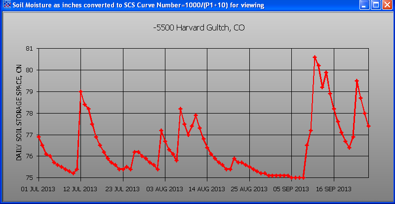
Note how the soil moisture hits CN_dry=75 on Sep 5. Reducing the CN_dry
would reduce the next peak flow which is way to high but may be a bad radar
adjustment. Also increasing the interception factor would help.
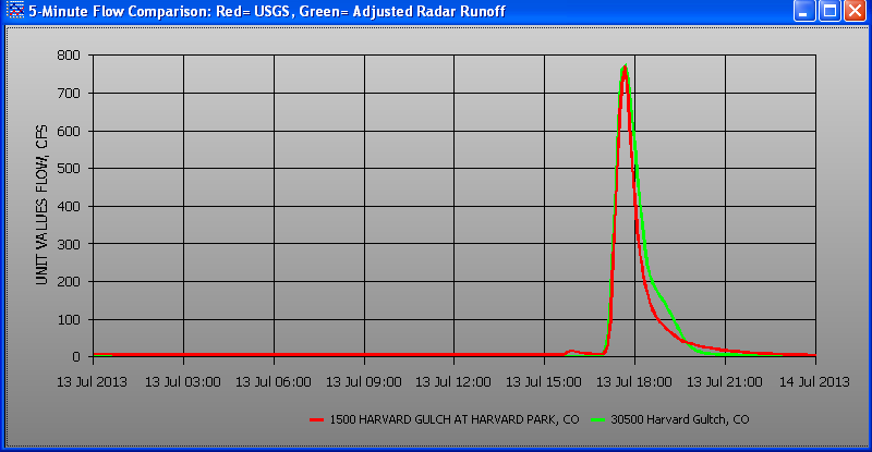
5-minute Hydrograph example
for July 13 (add my 3 triangle unit graph and adjust the ground water and I
could get this graph to fit like a glove but would it ever be accurate?).
If you're lag time is less than 4 times the 5-minute rainfall time-step you
better go to a Linear Reservoir because the unit-graphs can start flaking out.
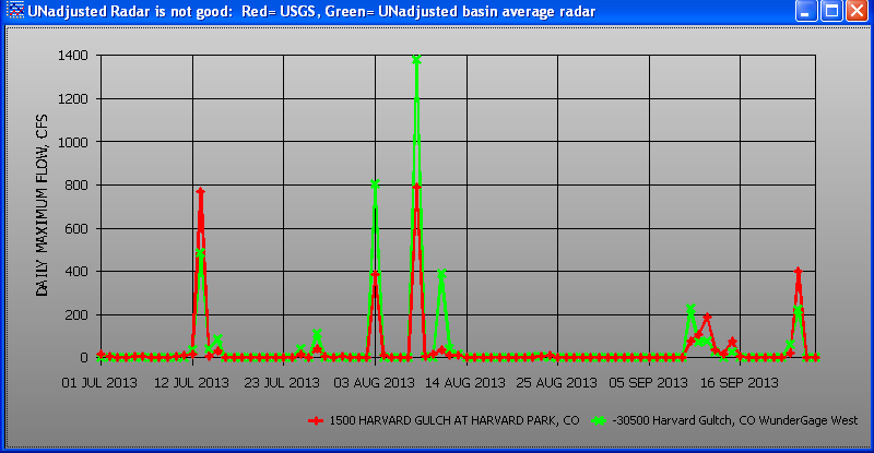
I'm rather pleased how well these
off-the-shelf cookbook parameters turned out for this site using adjusted radar
without costing us a dime. Below are the very ugly peak flow comparisons using
the Unadjusted Radar
5-minute rainfall record:
You are probably thinking like I did that using a single accurate
USGS rain gage would have worked out a lot better than messing aournd with
radar... Not so fast there...
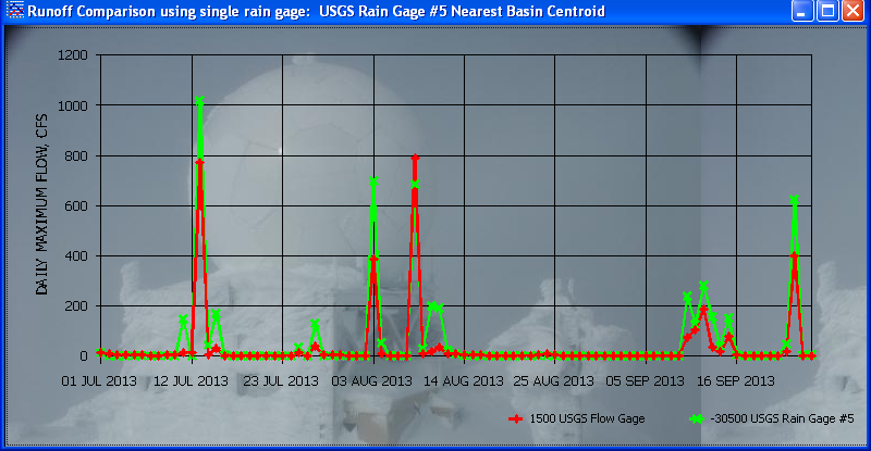
How about another single accurate USGS rain gage???
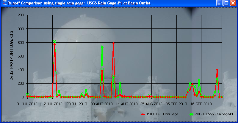
So now you must be thinking the average of 5 accurate USGS rain gages has to be
better than radar, right? We shall see about that...
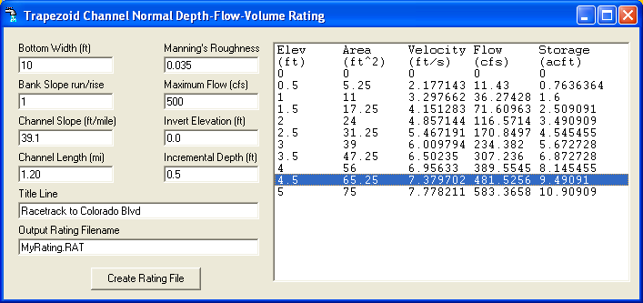
If you would like to
convert the computed runoff to flow depth at the USGS gage
then retrieve their rating table, paste it into Excel, delete the GH at zero
flow so zero flow has zero depth, reverse the depth, Flow columns, and using my
free GetRegression (on web page More Stuff) and select regression type Y=a(X-e)^b and you can get the equation for GetRealtime as (hint: select data
above depth=0.10):
GetRealtime_Setup.txt:
COMPUTE-Unit; 2500; Depth; Harvard Gultch, CO; 0;0;0.527493*(P1-0.09)^0.308399
and GetAccess Table rsite:
500; 2500; Harvard Gultch, CO; 2; depth; ft; feet; 30500; COMPUTE; 5; CO; 0
For complex ratings you can enter up to 5 equations
using lots of Pn parameters so see my Help web page for
other computation examples. Also you water quality gurus can add equations
for your sediment and who cares what else.
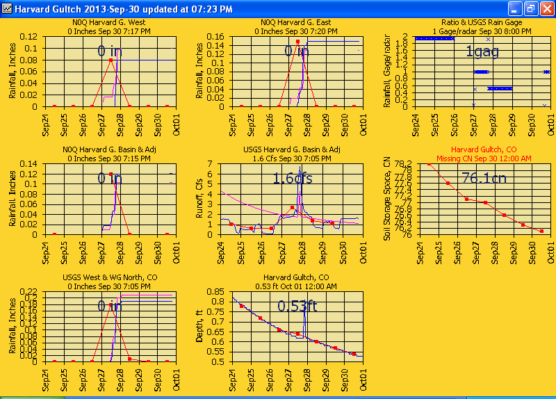
A GetGraphs page for viewing your real-time data or historical
periods:
Next will be a comparison of different radar adjustment strategies....
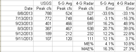
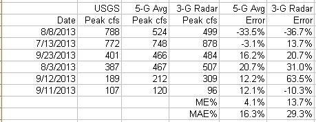
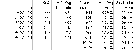
CAN RADAR BE BETTER THAN 5 USGS RAIN GAGES???
Here's a peek ahead. I think radar could be...
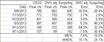
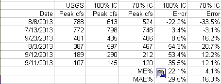
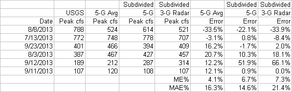
To evalutate differences in model results we will look at the
6 USGS peak flows
above 100 cfs and the model's error bias and error variability. Bias will be
mean of the errors (ME%) and variability will be mean of the unsigned errors
(MAE%) all in percent like this table for the graph above.
First,
because this is such a small basin, let's look at our N0Q radar cells used to average the basin rainfall:
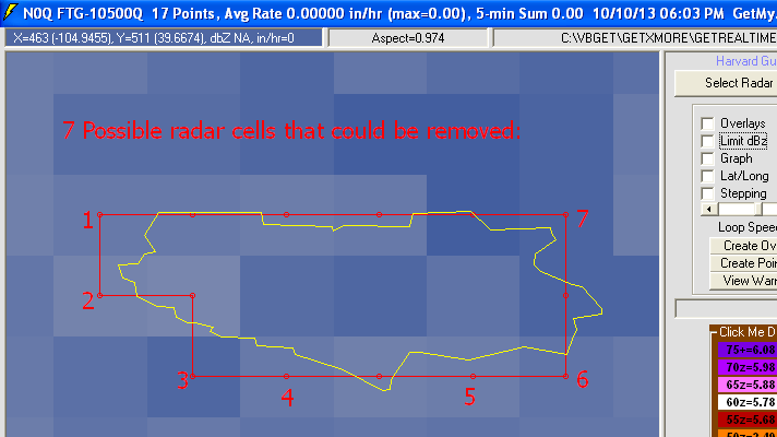
I note 7 possiple radar cells that may be hindering our basin average because
very little of these radar cell's area are within our basins boundary. Just
to be safe I will remove 1 cell at a time starting with cell #1 and see how our
peak flow compares with the USGS.
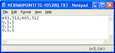
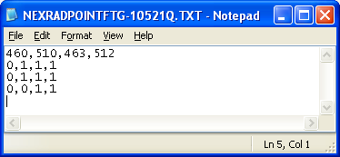
To remove a cell we edit the basin Point File: NEXRADPOINTFTG-10500Q.TXT
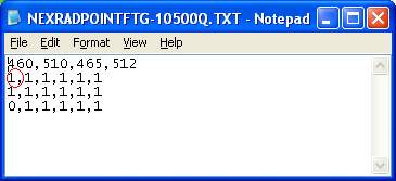
Radar cell #1 is x=460, y=510 from
screen top left and I will change the 1 to a 0.
That will make 16 radar cells that get averaged for the basin 5-minute rainfall.
Oh shoot! I would have to retrieve all the radar for 3 months with ech
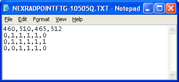
cell removal or create 7 new basin setup lines. On second thought I better
create a whole new site_id so I don't lose what I got and will just remove cells
1, 2, 3, 6, & 7 to give 12 cells remaining for basin averaging.
5 radar cells removed and saved as new Point File with new dsid:
The GetRealtime_setup.txt and table 'rsite' was updated but before I retrieve
all the radars again I had better plan ahead and see what other radar info may
be needed, like the radar at the 5 USGS gages:
-16500 06711575 H GULCH AT HARV PARK 39°40'18.20", 104°58'37.30"> 39.67172,
-104.977028
-12500 393938104572101 H G AT SLAVENS 39°39'38.99", 104°57'23.31>
39.66083, -104.956475
-13500 393947104555101 H G AT BRADLEY 39°39'46.50 104°55'53.58> 39.662916,
-104.93155
-14500 394028104560201 H G DENV ACAD 39°40'26.95 104°56'01.81>39.6741527,
-104.933836
-15500 394028104565501 H G AT UNIV PK 39°40'28.80 104°57'00.65> 39.674666,
-104.95018
and our
new 12 point basin: -10505
You may notice that I kept the same site_id=500 but used apparently different
datatype_id's. I did but I actually used the same DATATYPE_ID as 10
for all these rain gages. I try to use the XXYYY dsid as datatype_id + site_id
but with so many gages I threw that out the window here. And again I use a
negative dsid for radar and positive dsid for the rain gage data when I'm
thinking.
One caveat to creating DSID's willy nilly like I did here is that if your
site_id has a runoff computation with datatype_id=30, then it will automatically
overwrite 'rday' table values for DSID= 4xxx, -4xxx, and 5xxx where xxx=site_id.
4 is end of day soil space & precip sum and 5 is end of day groundwater storage.
If you wish to view these values in 'rday' then you have to add these 3 DSID's
to your 'rsite' table (or use SQL).
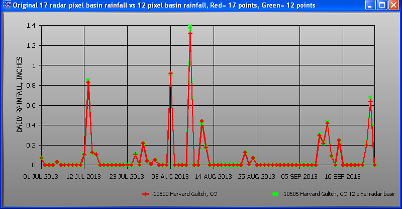
Hmmm... nothing to write home about here but does obey the law of areal
reduction. I'm sure glad I went all in at once instead of the grueling
agony of removing one cell out at a time.
But it did have more effect on the Peak Flows (no change to runoff parameters).
I'm wondering if I should re-calibrate on each rardar rain change or watch the
effect?
After more thought on how to proceed, recalibrating each case or not, I decided
to start with the full 5 USGS rain gage average (no radar) as the base
case (as did our benefactor's study), calibrate just it and not recalibrate the cases after that. This may be a
good choice here but my Charlotte, NC radar adjustments showed that:
Using 4 Wundergages at Charlotte, NC:
Best: 2 gages (east & west)
Nearly Best: 3 gages (east, west, & south)
Not very good: 4 gages (east, west, south, & north)
Pretty bad: 2 gages (south & north)
Very, very bad: 1 gage (south closest)
Very, very bad: 1 USGS gage (center of basin)
The Charlotte study was for a 32 sqmi basin with Wundergages all outside the
basin as far as 10 miles out. So more gages is not always better and 1 gage
should be avoided at all cost for larger basins. The Charlotte basin also
has 5 USGS rain gages within the basin, so after finishing up Harvard Gulch I
should probably look again at Charlotte using its USGS rain gages for adjustment
stategies.
Also the N0Q (0.6 mile) radar product proved superior to using the Very High
Resolution Level 2 (0.15 mile) radar product for adjusting radar. I
suspect the reason for this is trying to hit a rain gage from 10,000 feet up.
Using 4 nearest N0Q cells to a gage for adjustment was shown to be a bad idea at
my Las Vegas study. So trying to adjust the 4km NWS precip products would
be the equivelant to using 16 N0Q cells with 1 rain gage and seems pretty
preposterous. I am sure the NWS knows a heck of a lot more than I ever
will about
all this but they sure aren't telling me. Besides they use 6 hour time
steps.
Factoid: The very high resolution level 2 products for tornado wind
signitures are only available since 2011 and before that N0Q and Level 2
would be the same only their was no N0Q prior to that so use Level 2. Hey, I
don't run this show but praise be their is now N0Q images... although the NWS is
the last place to try and reliably get them in real-time...actually they don't
support post real-time either so I'm not quite sure how the NWS stays in
business... just use Iowa Mesonet... I think they're all in cahoots anyway.
If anyone has some web links to shed more light on all this please let me know
and I will add them here. But I get the feeling there is no 'grand unifying
theory' on weather radar adjustment at small basins and so every basin needs a
seperate study and why you should adjust your own radar yourself.
Now back to Harvard Gulth...
Well
the 5 USGS gage average runoff turned out poorly. I emailed the author of the lead
in article and he kindly responded with much needed basin info and also noted
what I have subsequently found which basically is, "I told you so"... meaning
this:
I thought the TR-55 manual
implies all kinds of adjustments to the curve number loss method are possible
for dealing with % of impervious running over pervious and such. This was some
what true with the Wundergage calibration, but not with the 5 USGS rain gage
calibrations. The CN had almost zero affect so it's not actually going to get
me anywhere fast using the CN curve number
methods. Note that the author used the EPA SWMM model in kinematic mode
with 59 sub-catchments divided along the lines of similar land uses and
developments with cascading planes for impervious areas.
Boy, 59 sub-catchments, that aint going to happen here BUT..., I added 'The Directly Connected Impervious Fraction'
to GetRealtime that the author discussed. This allows the fraction of the
%Impervious not dicrectly connected to be removed from the excess and added to
infiltration but limited by the Curve Number loss method. A 0.70 factor for
the % impervious connected really helped.
Improvement with Impervious Area fraction running over pervious area:
From Colorado Urban Drainage and Flood Control District for urban catchments studies. The
Levels in the graph are for the amount of Low Impact Development added between
the impervious areas and collecting channels. My calibrated 0.70 factor for 38% impervious shows some minimal low impact developments (Level
0).
The SCS Dimensionless Unit Graph's peak and recession was compared with other
unit graphs and I decided to go with the Linear Reservoir calibration here. The
SCS unit graph gave nearly identical results but I wanted to show those that
think the SCS unit graph is a poor choice for urban runoff that it can be fine
if your model allows adjusting soil and groundwater returns to give a proper
recession. Also once lag time becomes less than 4 or 5 times the 5-minute
rainfall time step, unit graphs may not fit the actual runoff very well on these
small catchments and the Linear Reservoir will do a better job.
Not that it's noticable for 3 months here but the
Linear Reservoir is a single step computation that is 100 times faster than
convoluting the other unit graphs and is something to remember when running 400
years of continous modeling... like we all do now and again.
The final 5 USGS rain gage average calibration wizard looks like this:
ADJUSTED RADAR COMPARISONS
5 USGS Rain Gage Radar Adjustment:
4 USGS Rain Gage Radar Adjustment (gages 2,3,4,5):
3 USGS Rain Gage Radar Adjustment (gages 1,3,5):

2 USGS Rain Gage Radar Adjustment (gages 1,3):
1 USGS Rain Gage Radar Adjustment (gage 2):
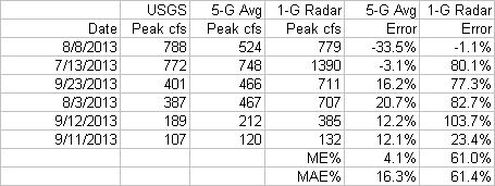
So much for my theory (wishful thinking) that radar would out perform 5 USGS
rain gages located within the basin. The graphs above do point out that 3,
4, 5 rain gage adjustmens are not too bad and the 3 gage adjustment looks like
something I could live with. 1 and 2 gage adjustments are to be avoided in
Colorado. Actually I would find another state to find work in hydrology
with these fast thunderstorms.
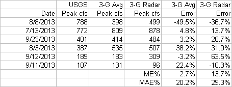
The 3 rain gage adjustment of basin radar is becomming a repeditive theme.
So would 3 gage adjusted radar be better than the average of the 3 USGS rain
gages??? Let's find out:
3 USGS Rain Gage Radar Adjustment (gages 1,3,5) versus 3 Gage Average:

Another thought is maybe the NWS is on to something with their 4km radar cell
precip products. A 4km cell is equivalent to the average of 16 N0Q 1km
cells used here. Perhaps minium basin size for using radar is 16
N0Q cells. This theory is based on the fact that radar error bias can
be very good but is higly variable so averaging multiple cells (basin size) or
time-steps (gage adjustments and storm duration) should improve accuracy.
A good case in point where precision can screw up your accuracy.
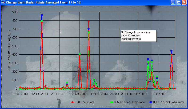
Using our original 17 point radar basin record seems to help as shown below.
I guess the next step in pursuing minimum radar cell count or basin size is to
sub-divide the 3.1 sqmi bain into upper and lower halfs at the other USGS flow
gage.
3 USGS Rain Gage Radar Adjustment (gages 1,3,5) of 12 Point and 17 Point
Basin Cells:
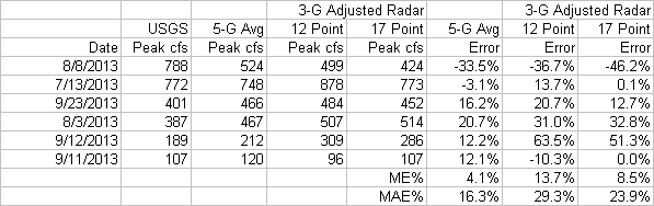
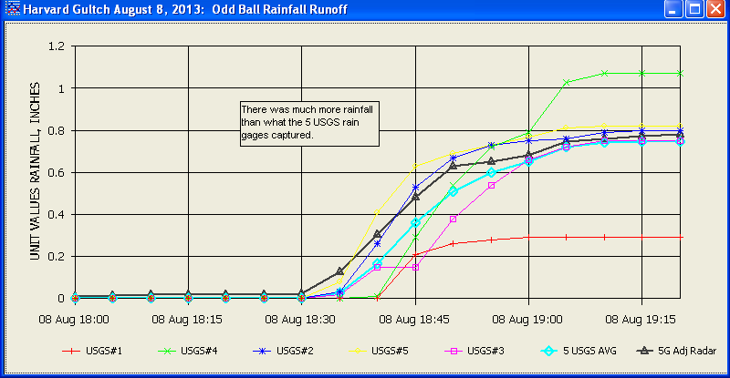
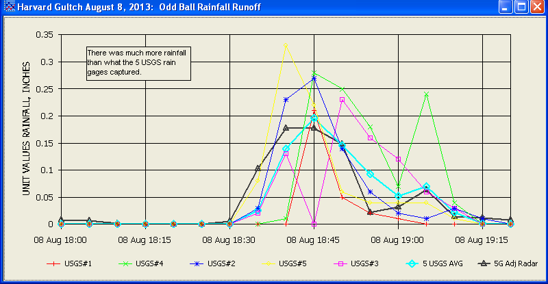
And why is August 8 so bad... sub-dividing the basin may help.
But I thought you said it wouldn't??? Cool your tamales, it won't.
A simple unit graph works until it doesn't. Is this a unit graph failure
or an excess rainfall failure.... or a USGS gaged flow failure. The gaged
flow looks fine... I think it's a gaged rainfall failure and radar could point
this out if you didn't have to adjust it with rain gages... ah the irony... but
failure at the highest peak flow is very unsettling and unless you get 1km wide
rain gages then you have to deal with sub stellar results just when you need
them most. Hmmm... would a 3 rain gage radar adjustment from all 3 rain
gages in the same radar cell help??? Probably not until it does. I
see a pattern here that is just life as we know it. What can go wrong,
does, and just at the peak... not a political statement. ;-0
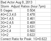
Using USGS 3 gages 2,4,5 actual average came very close to the August 8 peak but
using the same 3 gages to adjust the radar did not help at all. Using the
single gage ratio was correct for Aug 8 but was way to high for all the other
peaks.
Will sub-dividing the basin help???
Here are the sub-divided boundarys above and below the USGS gage at Colorado
Blvd:
Pixel Removal Sub Above Colorado Blvd:
and Sub Below Colorado Blvd:
Estimating loss
coefficients... Get out your cookbook from the top half of this web page above.
Above Colorado Blvd:
1.12 sqmi
C est for lag time on streets=26*0.015=0.39
Lag=0.16 hrs=9.6 min or 10 min=0.167 hours
CN= 1/4 commercial and 3/4 residential 1/4 acres CN= 92*.25+75*.75=79
%imperv=85%*.25+38%*.75=50%
CNc= CNp+(Pimp/100)*(98-CNp)*(1-0.5R)
from directly connected graph for Level=0.5, 50% gives 70% connected
Soil=B
CNc= 75+(50/100)*(98-75)*(1-.5*.3) CNc= 85
Below Coloradao Blvd:
2.01 sqmi
C est for lag time on streets & cobble channel 26*(0.015+0.035)/2 lag=0.5 hours
% imperv=1/4 acre Residential=38%
CNc=75+(38/100)*(98-75)*(1-0.5*0.3)
CNc= 82.4
Route Sub1 to USGS Gage at Harvard Park:
Using my free ChannelStorage.exe from my 'More Stuff' web page.
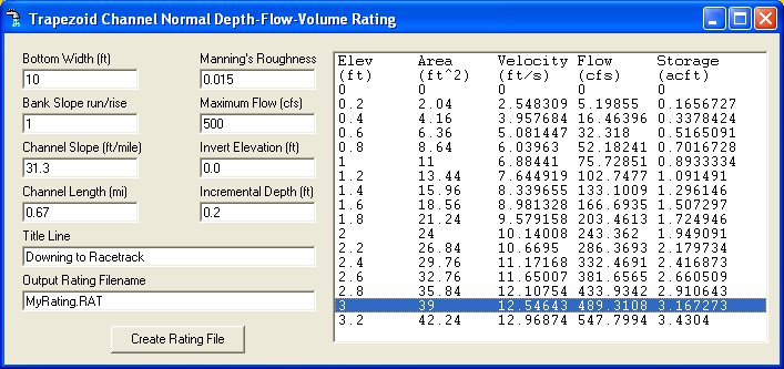
Channel going upstream from Downing Street at Elev0=5324
ft
0.67 miles n=0.015 trapazoidal 10' concrete Elev=5345 ft, at 500cfs=12.5 f/s
1.20 miles n=0.35 6' cut banks with cobbles Elev=5392 ft, at 500cfs=7.4 f/s
(0.67*12.5)+(1.2*7.4)/1.87=9.23 ft/s>>> 6.29 MPH
Travel Time= 1.87mi/6.29mph= 0.297hr=18minutes>>>20 minutes
Tatum and Muskingum
routing gave same peaks but I trust Tatum much more than Muskingum
but prefer Modpul but wasnt sure how to adjust it if it was wrong or how to
explain it.
Tatum's Travel Time=20 minutes
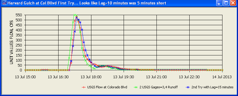
July 13
Sub1 Above Colorado Blvd. 2 USGS rain gages 3 & 4 (no radar) and reset
Lag to 15 minutes: Lag to 15 minutes:
Now the GetRealtime Routing file
and change 20 minute travel time to 15 minutes:
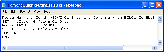
Route and Combined at Harvard Park USGS flow gage
and reset Lag=20 minutes, CNdry=75, %Impervious=30%, and directly connected=0.5... so
much for the cook book:
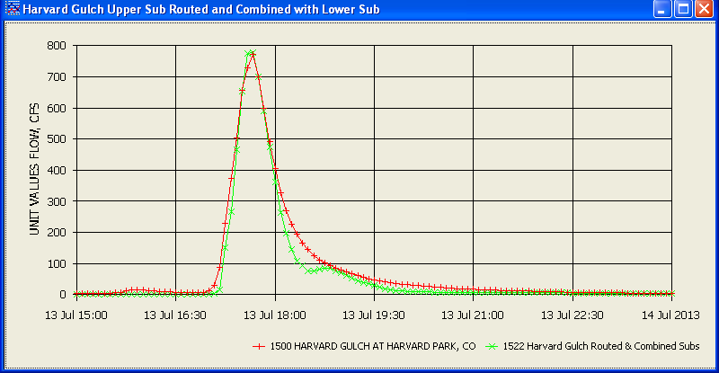
For the full season:
The August 8 problem for the subdivided upper 1.12 sqmi basin adjusted radar
with 6 cells is no better than 2 USGS rain gages.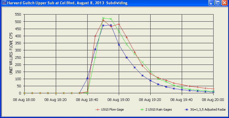
I was hoping the August 8 problem would be resolved in this upper Sub... not so.
I guess the lower Sub had rain everywhere but at the 3 lower gages or the wind
just blew the rain around them. Two rain gages per 1 sqmi is good at
Sub1, but 3 rain gages per 2 sqmi is poor at Sub2 but better than 3G adjusted
radar. I would just use 3G adjusted radar and start learning how to deal with it.
That way you can always blame the NWS for their help. ;-) Or as ol' Tom
from COE would be wont to say on Monday mornings... "Monkies could do runoff
studies using rain gages.", hey Tom!
Now to add the whole season of 3G adjusted and subdivided
radar. radar.
But what if you only had 3 Wundergages OUTSIDE your
basin... then adjusted radar might start looking betther than Nothing.
Epilog: I got a good lesson in cascading planes and that was well worth
the effort here. Colorado thunderstorms are best left to the experts!
I have not seen storms out of nowhere going in 10 directions since watching a
lava lamp in the 60's. I'm off to do
nothing in Arizona where at least there... the pay's better.
----------------------------------------------------------------------------------------------------------
Additional page links about
ET, Runoff, and Nexrad Radar help and comparisons:
List of How To Videos on Youtube
Help Page for GetNexrad.exe
Nexrad Rainfall to Tipping Bucket Comparison
(how I got started)
ET and Radar Rainfall along the Lower Colorado
River, AZ-CA
Nexrad Rainfall-Runoff Comparison Las Vegas
Valley, NV w/ runoff setup & radar adjustment
Nexrad
Rainfall-Runoff Comparison San Jouqin Valley, CA w/snowmelt and radar adjustment
Nexrad
Rainfall-Runoff Comparisons in northwestern Arizona
Nexrad Snowfall Comparisons in western
central Sierras, CA
Nexrad
Rainfall-Runoff Comparison Beech Mtn, NC w/snowmelt and radar adjustment
Radar Rainfall
Ajustment, Charlotte, NC
WEBSITE MAP


WU USGS USBR NWS GoC USCS
CWRD COE CWRD COE
More Free Downloads
Comments/Questions
Contact Me
Label
|
|